Building a Suspension Kinematics Simulation Tool: Part I

I would have written you a shorter letter…

Background

A couple of years ago, I stumbled across SolveSpace, a free, parametric CAD system with one feature that’s pretty unusual for a user-facing CAD tool: it also ships as a library, so you don’t need to run the GUI to use it. As someone who had once spent much of their working day thinking about suspension systems, this grabbed my attention, and I wondered if I could use SolveSpace’s geometric constraint system to build a tool that would simulate the kinematic behaviour of the sort of double wishbone suspension systems you typically see on open-wheel racing cars.

Specialist commercial systems do exist for this sort of thing, and many automotive and motorsport engineering teams are likely using tools like OptimumKinematics and Lotus Shark to help design their cars, though engineering software no longer appears to be an avenue of business Lotus are pursuing.

My first-hand experience is limited to internally developed systems which I had no hand in writing, but which I was always impressed by.

Lotus Shark in action:

The SolveSpace system

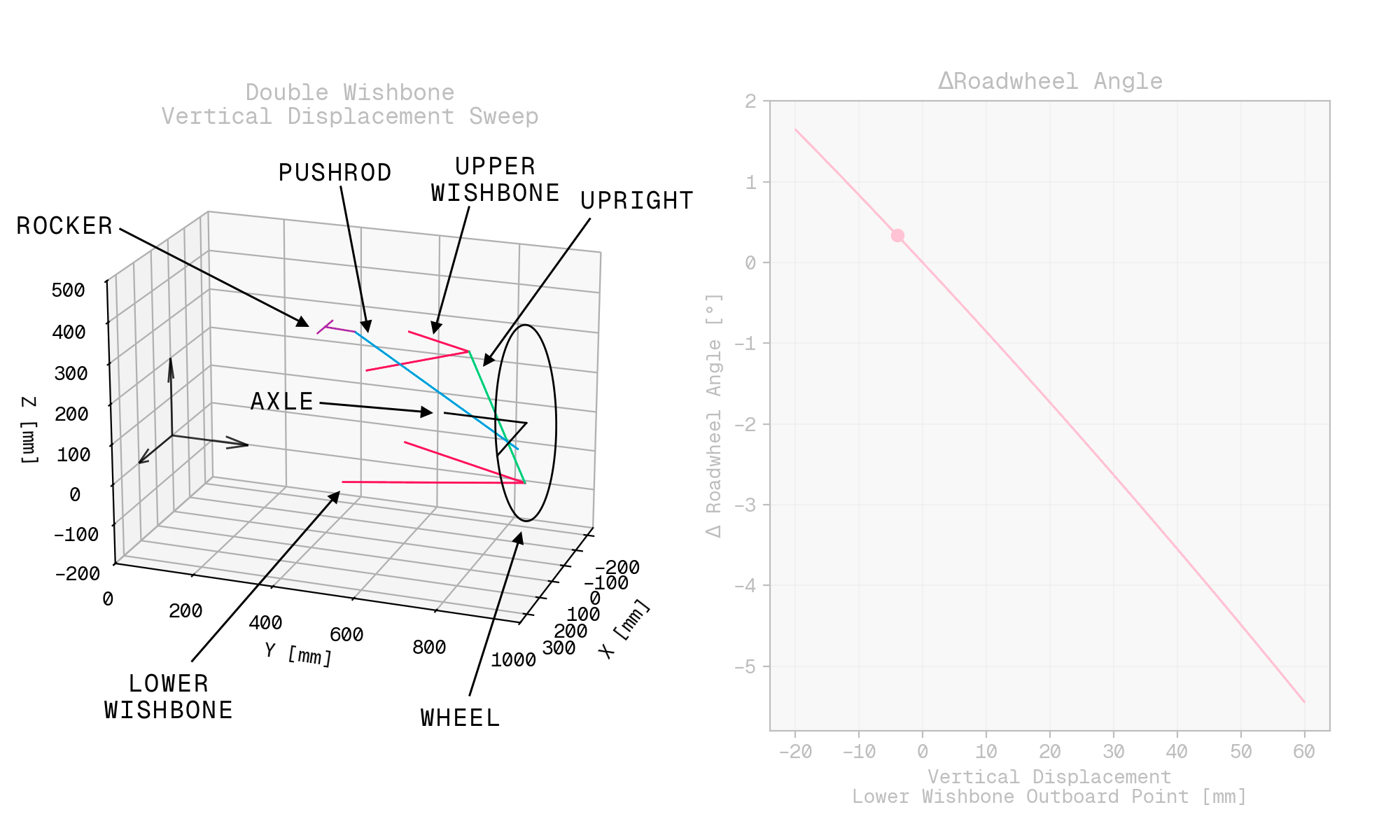
Commercial systems aside, I spent a day or two over the Christmas holidays hustling together a tool using python_solvespace, and eventually wound up with something I could use to run a sweep of vertical hub displacement on a familiar sort of suspension layout: a double wishbone corner arrangement with an upright-mounted pushrod and an inboard rocker.

From the solve positions, I was then able to work out the sort of parameters a vehicle dynamicist might actually be interested in, e.g., how much the roadwheel rotates about the kingpin axis during vertical suspension displacement, otherwise known as bump steer.

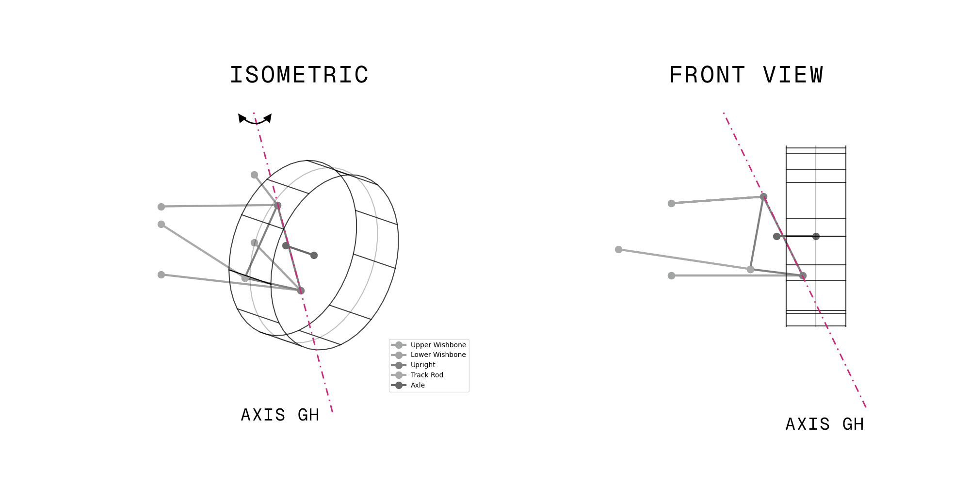
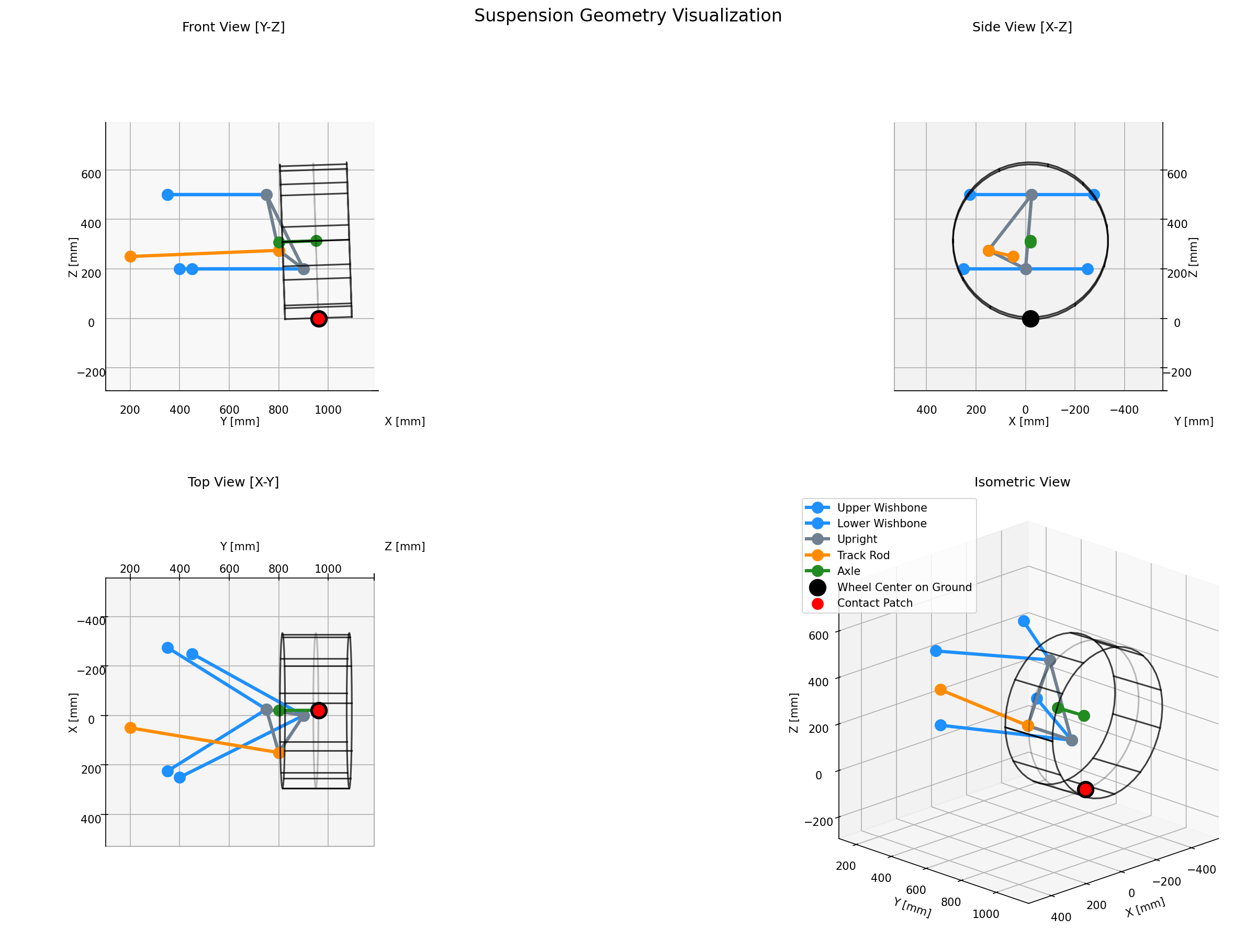
Since the matplotlib visualisation isn’t going to win any awards any time soon, here’s an annotated version that highlights each of the elements in the system.

If you’re into that sort of thing, here’s the waffle that I posted on the worst website on the internet at the time:

• https://www.linkedin.com/feed/update/urn:li:activity:7010361380478296064/
• https://www.linkedin.com/feed/update/urn:li:activity:7018680493319614465/

I’m not going to share any of the code for this because A) it’s awful and B) it’s just using the SolveSpace library, so nothing too interesting to show there. It also involved some additional juggling with Rodrigues’ formula and so on, which I felt shouldn’t be required.

However, the experience did make me curious as to whether or not I could roll a system like this myself.

DIY system basics

A year on from when I first discovered SolveSpace, at the next Christmas break, I figured I would have a stab at building a geometric constraint solver of my own.

At the outset, I thought this would be an interesting application for Google’s JAX library. I’ve written about the appeal of automatic differentiation before, and in the context of suspension kinematics, engineers are often interested not only in the positions of parts of the suspension, but also how those positions change with respect to other things; ratios and gradients. Plus, if going down the route of a numerical solver, gradients are always useful.

So, without thoroughly reading the JAX^† docs, I set about it…

^†Something I would come to regret. It turns out that JAX requires some not insignificant considerations to be made up front, and trying to patch it into a system after you’ve built most of it is… non-trivial.

Problem statement

Automatic differentation aside, it’s worth stating the core problem being tackled here:

Given a suspension system modeled as a collection of rigid bodies (chassis, wishbones, uprights) connected by ideal spherical joints, we want to solve for the complete kinematic state of the system.

Objective:

For any given configuration defined by our boundary conditions, determine the unique positions and orientations of all bodies and connection points in the system.

Known conditions:

• There are fixed geometric relationships between connection points on each rigid body.
• There are kinematic constraints at each spherical joint; each joint connects two specific points, one on each body.
• Boundary conditions include specified position/orientation of one or more bodies, e.g., chassis is fixed, wheel centre sits at a prescribed Z position, trackrod inboard point sits at a prescribed Y position.

Key assumptions:

• For every sweep step, the constraints yield exactly one feasible configuration; there are no missing or inconsistent constraints.
• All bodies are perfectly rigid.
• All joints are ideal spherical joints (3 rotational DOF, 0 translational DOF).

More on knowns and assumptions

Irrespective of how we go about finding the values we’re interested in, we can lean on what we know about the system to build a mental picture of what we need to solve, and then to help steer the approach we opt for.

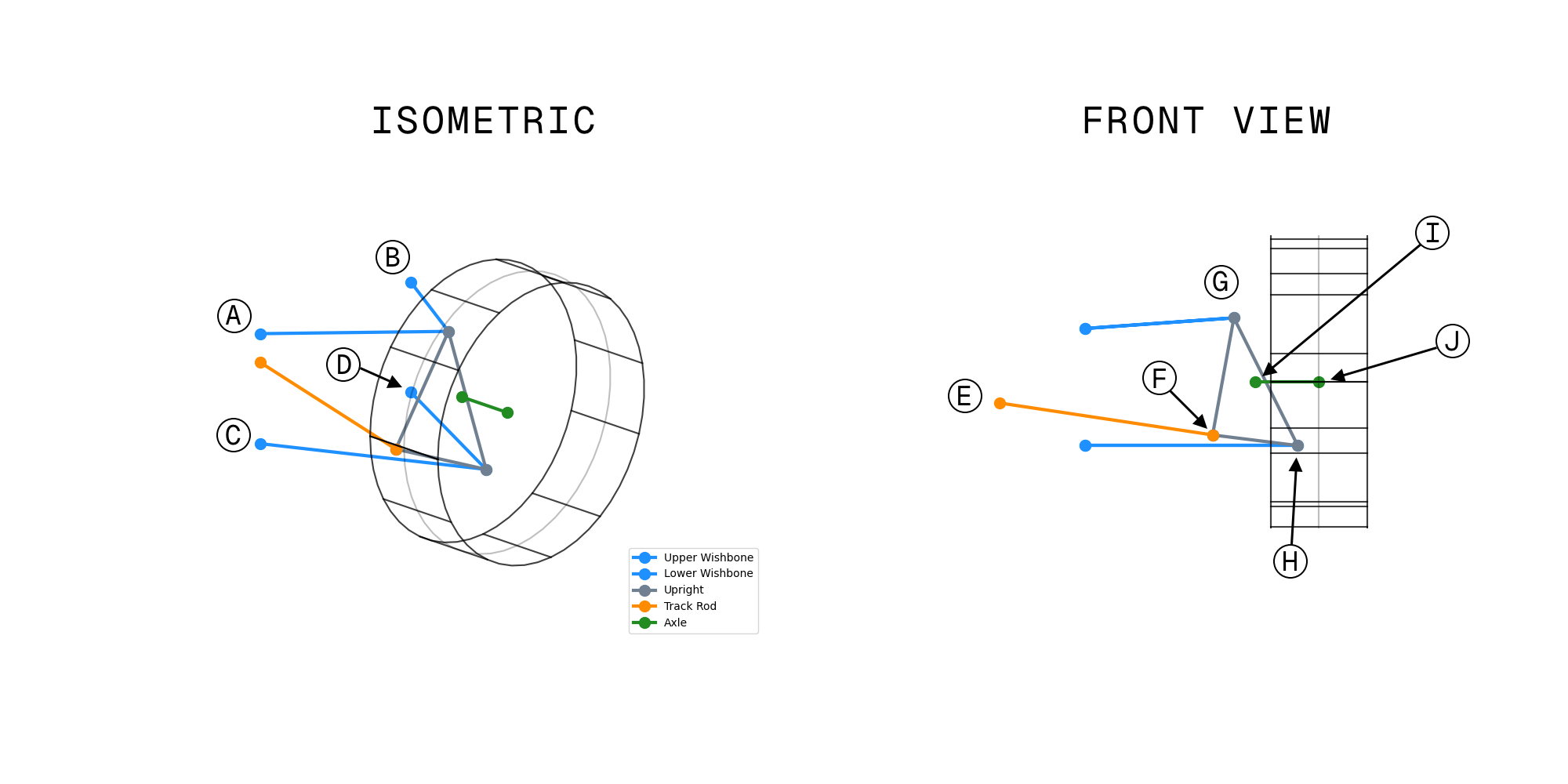
Mapping our knowns and assumptions more concretely to the points we’ll be dealing with, as shown in the figure below, we can say that:

1. Wishbone inboard points $A$, $B$, $C$, and $D$ are all fixed to the chassis.
   • They are effectively grounded; we will consider the chassis to be fixed in space.
2. Points $A$ and $B$ effectively form the axis about which the top wishbone can rotate.
3. Points $C$ and $D$ effectively form the axis about which the bottom wishbone can rotate.
4. Top wishbone outboard point $G$ will hold constant respective Euclidean distance from points $A$ and $B$.
5. Bottom wishbone outboard point $H$ will hold constant respective Euclidean distance from points $C$ and $D$.
6. The upright can be described by points $F$, $G$, and $H$, and the Euclidean distance between each pair of these points will remain constant.
7. Points $G$ and $H$ effectively form the kingpin axis, i.e., the axis about which the upright can rotate.
8. For a given rack displacement, the trackrod inboard point $E$ can be considered fixed.
9. The Euclidean distance between points $E$ and $F$ will remain constant.
10. The axle, described by points $I$ and $J$, is rigidly fixed to the upright.

Note also that:

• Point $G$ refers to both upper wishbone outboard point and upright top mount, i.e., the upper balljoint.
• Point $H$ refers to both lower wishbone outboard point and upright bottom mount, i.e., the lower balljoint.
• Point $F$ refers to both trackrod end point and its mount on the upright, i.e., the outer trackrod end (TRE).

Each of these point pairs is considered to be coincident.

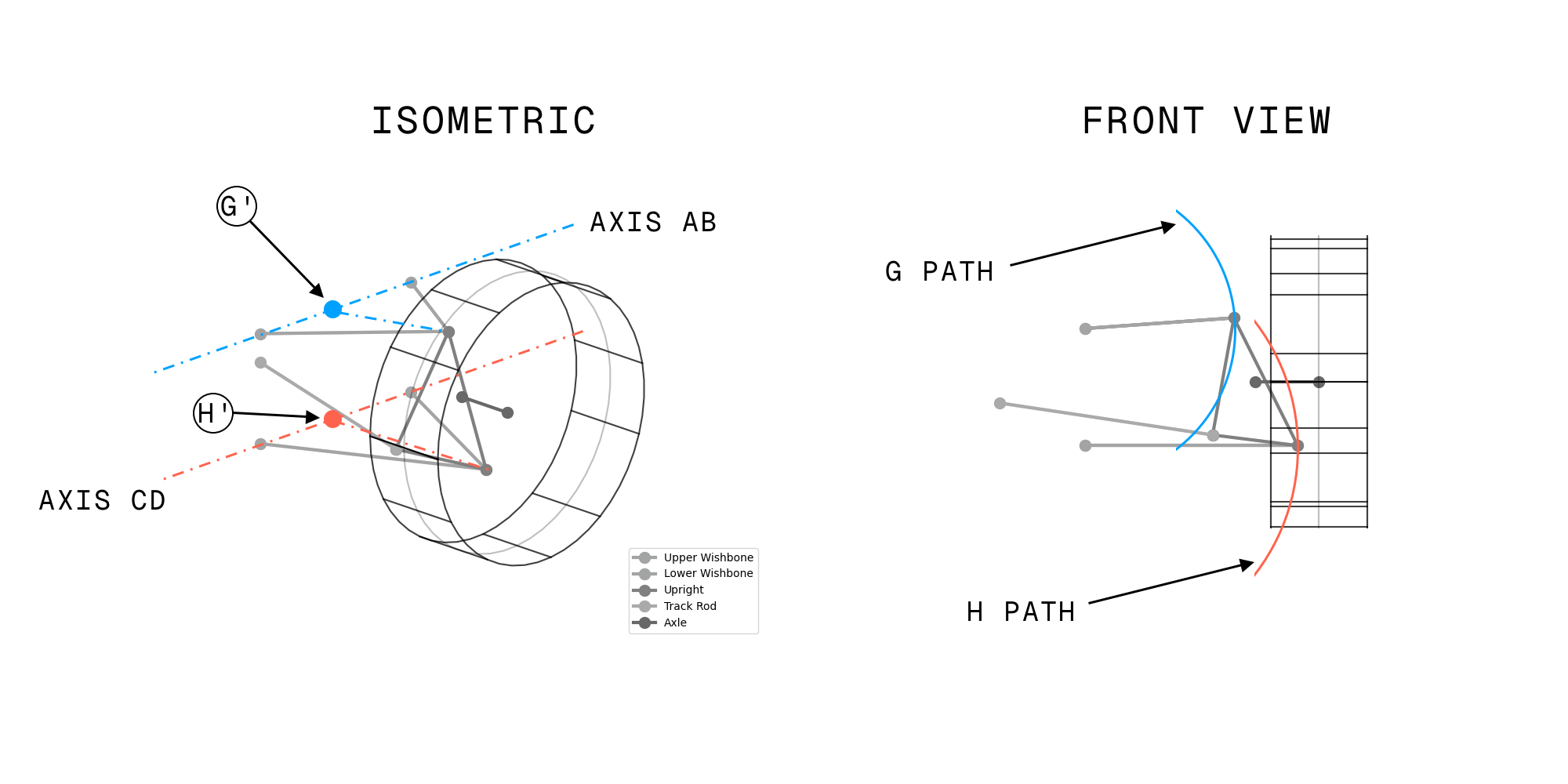
Considering what we know about the system at this point, a few more characteristics of the system’s behaviour can be intuited:

• The path followed by the upper wishbone outboard point, $G$, traces a circular arc across a plane that is perpendicular to the axis $\vec{AB}$ and which passes through $G$. The arc’s centre point, $G^\prime$, lies on the vector $\vec{AB}$, and its radius is the distance from $G$ to $\vec{AB}$.
• Similarly, the path followed by the lower wishbone outboard point, $H$, traces a circular arc across a plane that is perpendicular to the axis $\vec{CD}$ and which passes through $H$. The arc’s centre point, $H^\prime$, lies on the vector $\vec{CD}$, and its radius is the distance from $H$ to $\vec{CD}$.
• The upright and wheel assembly effectively form a rigid body which may, rack permitting, rotate about axis $\vec{GH}$.

I find it easier to imagine the system than reason entirely about symbolic mathematics, so the two figures below should help illustrate the degrees of freedom that the system has.

Possible approaches

At a high level, there are really two ways to go about meeting our objective. Positions and orientations could be determined with an analytical method, or with a numerical method.

At the time, I didn’t really give much consideration to an analytical approach; this is the sort of problem that I figured would be difficult to hammer out symbolically, and likely very inflexible^† even then. A numerical method, however, would be both well suited and flexible. Plus, I’ve always enjoyed working on optimisation problems, which this sort of thing would share a lot of DNA with.

^†What I mean by flexibility here is really having the ability to drive the simulation based on a selection of parameters. Maybe you want to solve for all of the positions in the system at a given wheel centre Z height, but maybe you want a given lower balljoint position, or upper balljoint position. With an analytical approach, you would need different equations with different subject terms to achieve this. Practically, I suspect you would probably end up building one solution path then reinterpolating it onto your desired breakpoints when you wanted something else… which feels like it violates the analytical purity.

Conversely, a numerical method will just have a bunch of error terms which we can define, and we can choose which is our driving target, so we can more or less do whatever we want without having to do anymore algebra; the solver will work it out for us.

Analytical

In 2D, the front-view of a simple double wishbone arrangement is effectively a four-bar linkage, for which a closed-form solution exists; you can just solve all the trig.

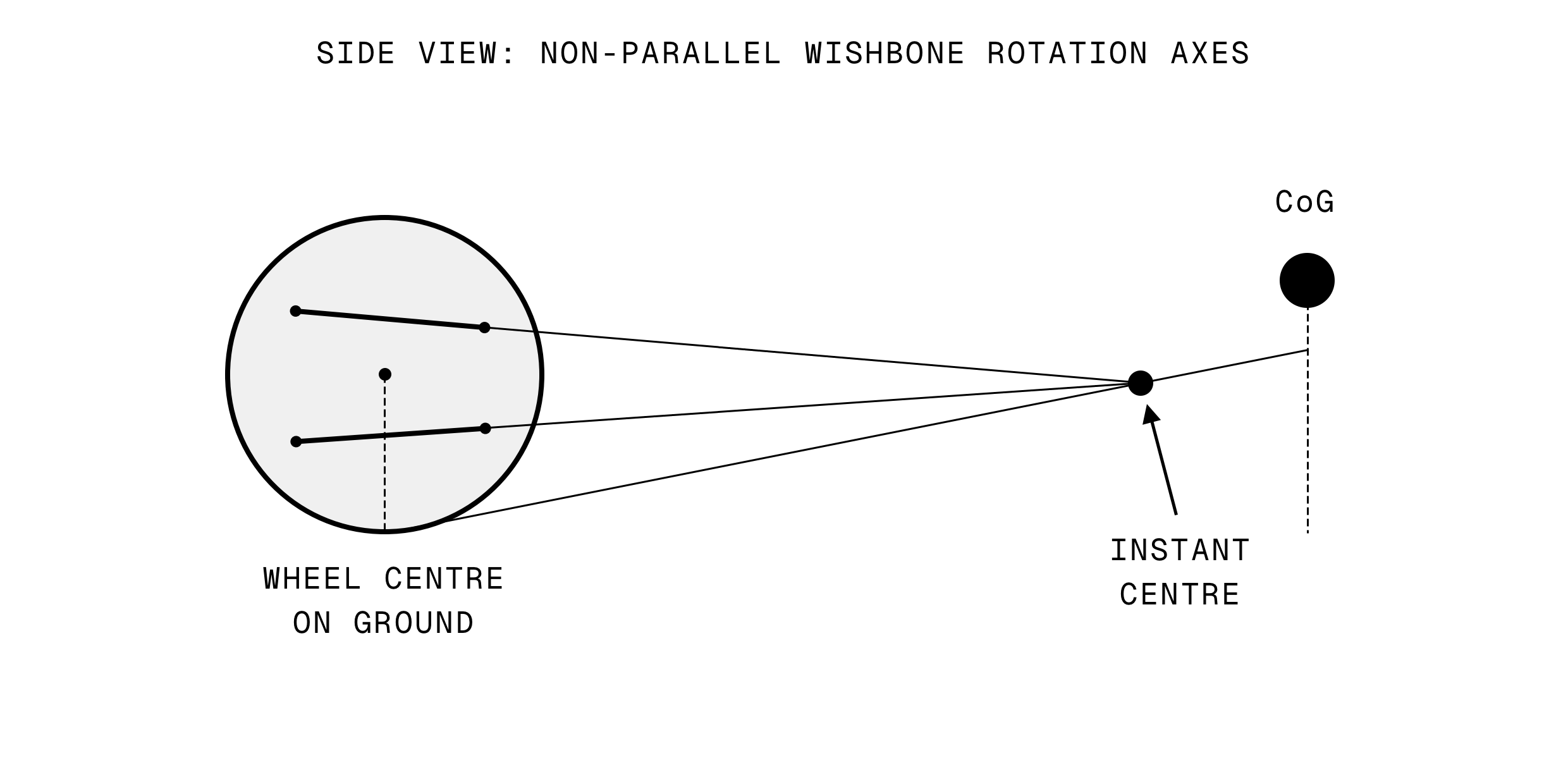
This approach could be applied to the 3D scenario provided that, in side-view, a line struck between the inboard points of your upper wishbone would be parallel with a line struck between the inboard points of your lower wishbone.

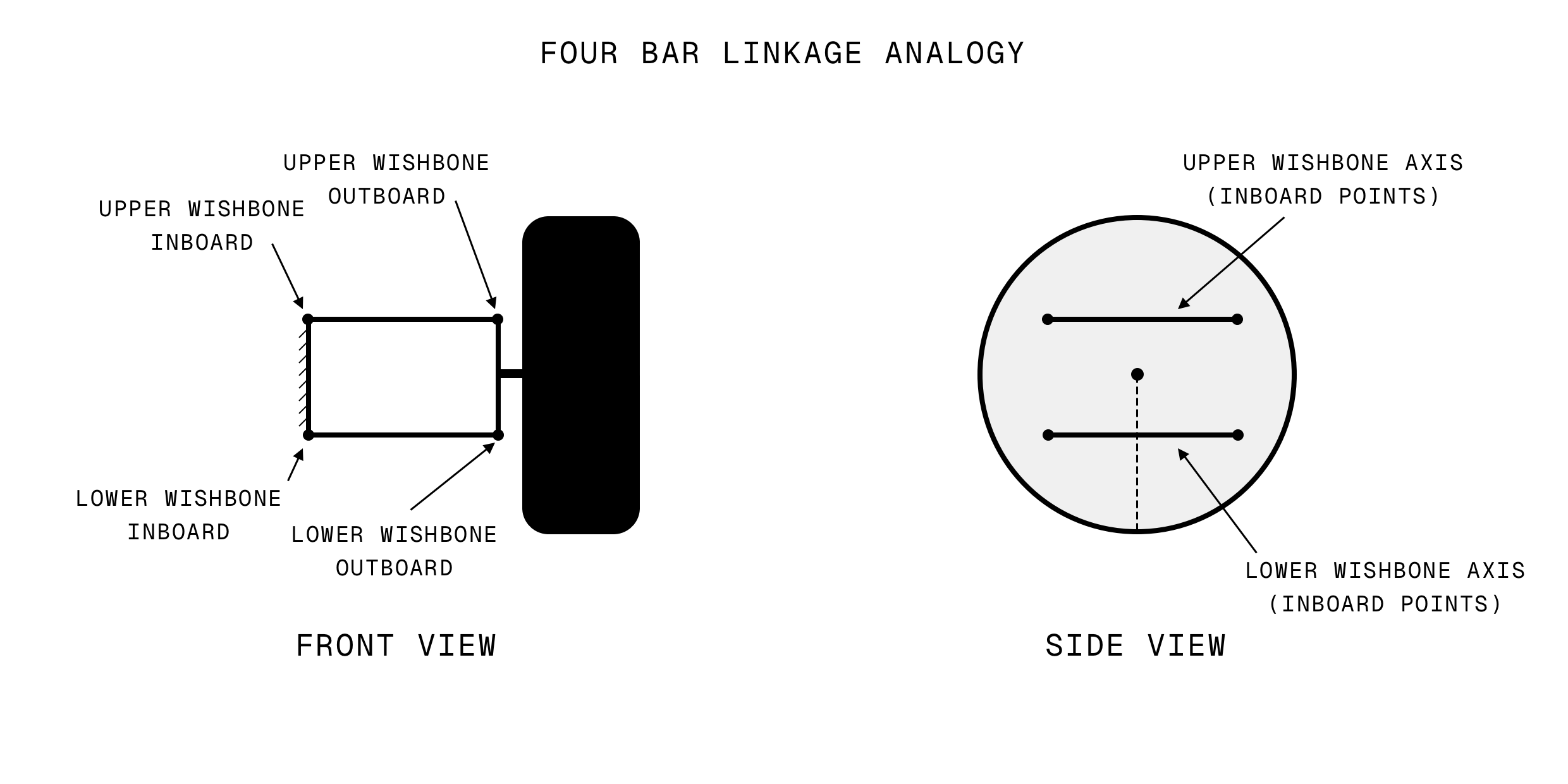
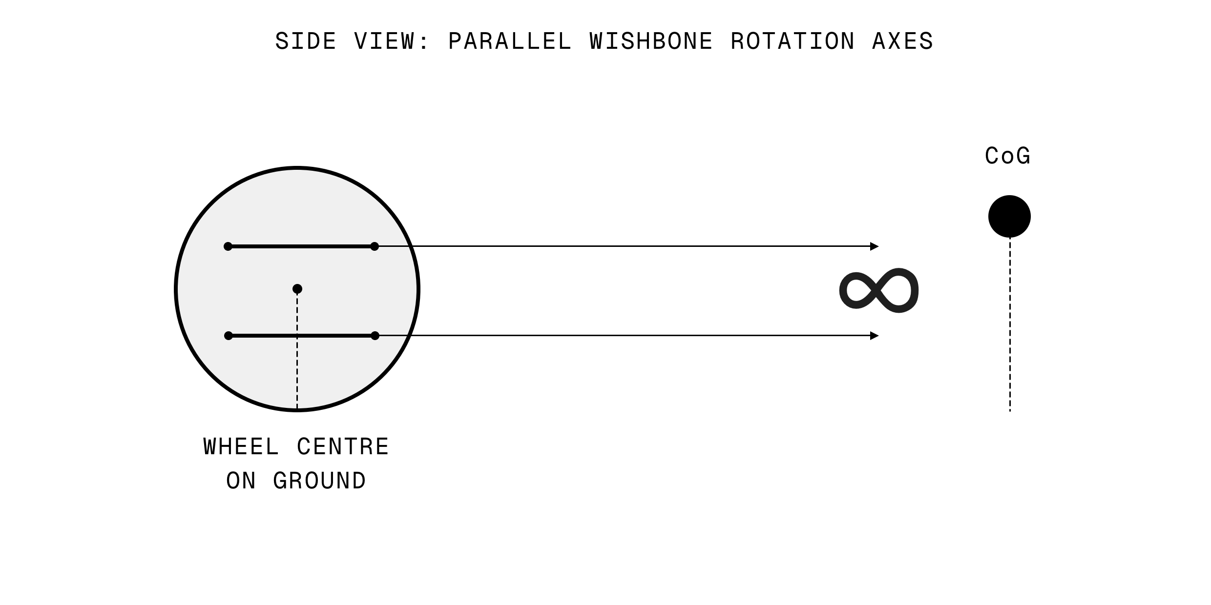
While this probably is the case for some suspension systems with this layout, imposing it as a constraint on your suspension design would mean that your side-view instant centre would lie at infinity, so you could not design a system with any geometric anti-squat or anti-dive characteristics. This would be a significant limitation, and obviously prevent the analysis of many real suspension systems which do have these traits.

Given that the four bar linkage analogy does not have legs, a more sophisticated method would be required for any analytical approach.

Practically, we could go about this by leaning on what we know about the system from our knowns and assumptions above. Adopting some new variable names that should be a little bit easier to reason about than point identifiers, we have the following known constants which are either system inputs or can be computed directly from those inputs:

1. $a_u$: upper wishbone rotation axis, $\vec{AB}$.
2. $x_u$: a known point on the upper wishbone rotation axis, e.g., $A$ or $B$.
3. $o_u$: upper wishbone outboard point / upper balljoint, $G$.
4. $c_u$: upper wishbone arc centre point, $G^\prime$.
5. $r_u$: vector from known point on the upper wishbone axis to outboard point, $\vec{x_u G}$.
6. $R_u$: distance from upper wishbone rotation axis to outboard point, $\lvert\vec{G^\prime G}\rvert$.
7. $a_l$: lower wishbone rotation axis, $\vec{CD}$.
8. $x_l$: a known point on the lower wishbone rotation axis, e.g., $C$ or $D$.
9. $o_l$: lower wishbone outboard point / lower balljoint, $H$.
10. $c_l$: lower wishbone arc centre point, $H^\prime$.
11. $r_l$: vector from known point on the lower wishbone axis to outboard point, $\vec{x_l H}$.
12. $R_l$: distance from lower wishbone rotation axis to outboard point, $\lvert\vec{H^\prime H}\rvert$.
13. $L_{kp}$: distance between upper and lower balljoints; kingpin length, $\lvert\vec{GH}\rvert$.
14. $L_{tr}$: trackrod length, from inner (rack) TRE to outer (upright) TRE, $\lvert\vec{EF}\lvert$.

Ignoring steering for the time being, that leaves us with just two unknowns to solve for, one of which we will use to drive the system:

1. $\theta _u$: upper wishbone angular displacement.
2. $\theta _l$: lower wishbone angular displacement.

On the face of it, this isn’t too bad. There’s a process we’ll be able to work through to solve for these values:

• A) Each outer balljoint moves on a circular arc. Leverage this to find:
  • The equations that describe each of these circles.
  • The equation that yields the position of a given outer balljoint at a specified $\theta$ value.
• B) Enforce constant kingpin length, $L_{kp}$. At a given $\theta$, since one balljoint position is already known, this can be established via circle-sphere intersection.
  • The ‘free’ balljoint must lie on the previously established circular arc.
  • The kingpin axis has one point fixed at the known balljoint position, but its other extreme could lie at any point on a sphere of radius $L_{kp}$ whose centre lies at the known balljoint position.
• C) Using known outer balljoint positions, solve for all remaining unknowns.
  • Now that the pose of the system is known, you can use vanilla trigonometry to work out where all your points live, and start calculating whatever else you’re interested in: camber, caster, antis etc.

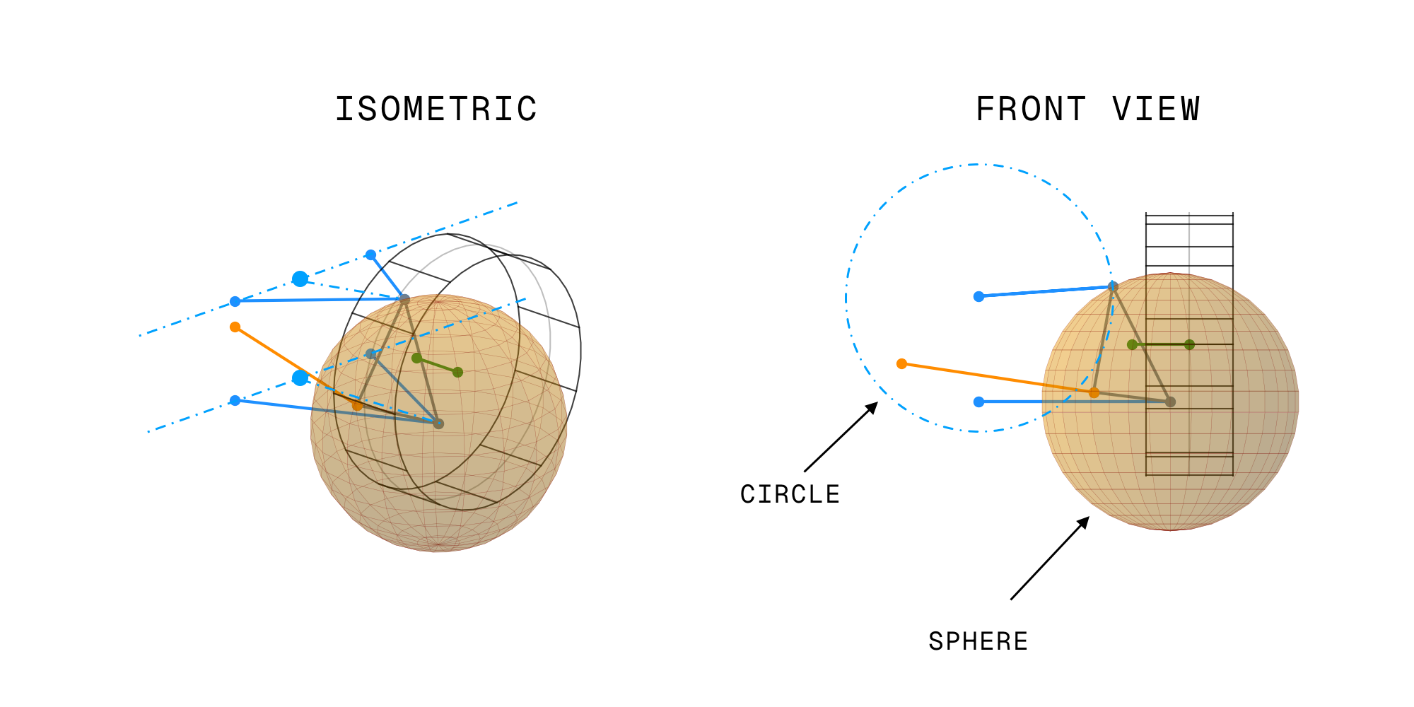
The figure below shows broadly what we mean by circle-sphere intersection. For a known lower wishbone angle, $\theta _l$, we know that the upright could, provided it doesn’t bump into anything, be oriented to leave the upper balljoint point lying anywhere on the sphere’s surface. However, we also know that our upper balljoint has to follow the arc prescribed by the upper wishbone. Assuming our upright is actually connected to both wishbones, we can see that the upper balljoint must lie at the intersection of the circle and the sphere.

We could of course work from the top wishbone, place the sphere at the top balljoint, and imagine our circle being drawn around the lower wishbone axis; the convention is our choice.

Fair warning, this is likely to be riddled with errors, but I think the maths here would shake out something like this, assuming we’re driving the system with a known lower wishbone angle, $\theta _l$.

A) Parameterise the upper circle:

As noted above, our intuition is that $G^\prime$ defines the arc’s centre. Analytically, to trace the upper balljoint’s path we consider its relationship to the wishbone’s rotation axis. If we let $x_u$ be a known point on the axis (e.g., one of the inboard points), the offset vector from this axis point to the outer balljoint is:

$$r_u = o_u - x_u$$

We can decompose this into two components:

$$r_u = (r_u \cdot a_u) a_u + r_{u\perp}$$

Where:

• $(r_u \cdot a_u) a_u$ is a component parallel to the rotation axis.
• $r_{u\perp}$ is a component perpendicular to the rotation axis.

Since the wishbone rotates around the axis $a_u$, only the perpendicular component really matters for the circular motion; the parallel component just tells us how far along the axis the plane on which the circle is drawn sits. In the simple case, where the wishbone forms an isosceles triangle when viewed from above, this would be half way between the two inboard points.

Note that the radius of the circular path, $R_u$, is simply the length of this vector: $||r_{u\perp}||$.

Now we can set up a coordinate system for the circle. The circle’s centre lies on the rotation axis at a position we can call $c_u$. This is the projection of $o_u$ onto the axis:

$$c_u = x_u + (r_u \cdot a_u)a_u$$

We create two perpendicular unit vectors ($u_u$ and $v_u$) that lie in the plane of the circle, allowing us to parameterise any point on the circle using the angle $\theta_u$:

$$u_u = \frac{r_{u\perp}}{||r_{u\perp}||}$$

$$v_u = a_u \times u_u$$

Note that for $u_u$ and $v_u$ to be computed like this, $a_u$ must be normalised to be a unit vector. The cross product here ensures that $v_u$ is perpendicular to both $a_u$ and $u_u$.

This should help illustrate the setup. Note that $x_u$ is drawn at an arbitrary position on the axis to make the vector $r_u$ visible, but in a practical scenario $x_u$ would likely be a known inboard point.

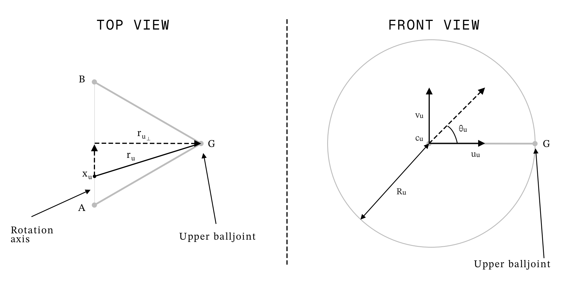
Once we’ve cranked through all of that, a point on the circle is given by:

$$p(\theta_u) = c_u + R_u (u_u \cos\theta_u + v_u \sin\theta_u)$$

Note that we really only need $u_u$ and $v_u$ because our wishbone’s axis of rotation doesn’t necessarily align with any of the axes in our global coordinate system. Our basis vectors, $u_u$ and $v_u$, effectively define a local coordinate system in the plane of the circle.

B) Enforce constant kingpin length:

The key insight here is that the upper and lower balljoints must always be exactly $L_{kp}$ apart. Since we know, or can trivially compute, where the lower balljoint is for a given $\theta_l$, the upper balljoint must lie on both:

1. The circular arc defined by the upper wishbone, and,
2. A sphere of radius $L_{kp}$ centred at the lower balljoint.

The intersection of this circle and sphere gives us our solution.

For the known lower balljoint position, $q(\theta_l)$, we want to enforce:

$$||p(\theta_u) - q||^2 = L_{kp}^2$$

So, if we define vector from the lower balljoint to the upper circle centre:

$$d_{uq} = c_u - q$$

We can then expand the constraint equation:

$$||d_{uq} + R_u(u_u \cos\theta_u + v_u \sin\theta_u)||^2 = L_{kp}^2$$

Because $u_u$ and $v_u$ are perpendicular unit vectors, this expands to:

$$||d_{uq}||^2 + 2R_u [(d_{uq} \cdot u_u)\cos\theta_u + (d_{uq} \cdot v_u)\sin\theta_u] + R_u^2 = L_{kp}^2$$

Rearranging into standard trigonometric form:

$$A\cos\theta_u + B\sin\theta_u + C = 0$$

Where:

$$A = 2R_u (d_{uq} \cdot u_u)$$

$$B = 2R_u (d_{uq} \cdot v_u)$$

$$C = ||d_{uq}||^2 + R_u^2 - L_{kp}^2$$

In this system:

• $A$ represents how much the constraint error depends on the cosine component of the upper wishbone’s rotation. It is proportional to how the vector from the lower balljoint to the circle centre projects onto $u_u$, the first basis vector of the local coordinate frame in the circle’s plane, i.e., the direction along which $\cos\theta_u$ moves the balljoint around the circle.
• $B$ represents how much the constraint error depends on the sine component of the upper wishbone’s rotation. It’s proportional to how that same vector projects onto $v_u$, the second basis vector of the same local coordinate frame, i.e., the direction along which $\sin\theta_u$ moves the balljoint around the circle.
• $C$ represents the part of the squared distance constraint that is independent of the upper wishbone’s rotation angle, $\theta_u$. Its value, $C = ||d_{uq}||^2 + R_u^2 - L_{kp}^2$, sets the target that the angle-dependent terms must meet, as the full equation is $A\cos\theta_u + B\sin\theta_u = -C$. A real geometric solution is possible only if this target value is achievable, which occurs when $|C| \le \sqrt{A^2+B^2}$. A non-zero value for $C$ is typical for any viable configuration.

C) Solve for remaining unknowns:

We now have a linear combination of sines and cosines equal to a constant. We can solve this using a standard trigonometric identity. First, we convert the linear combination into a single cosine function:

$$R = \sqrt{A^2+B^2}$$

$$\phi = \text{atan2}(B,A)$$

This allows us to rewrite our equation as:

$$A\cos\theta_u + B\sin\theta_u = R\cos(\theta_u - \phi)$$

So our constraint becomes:

$$\cos(\theta_u - \phi) = -\frac{C}{R}$$

Provided $|C| \le R$ (meaning a solution exists geometrically), the solutions are:

$$\theta_u = \phi \pm \arccos(-\frac{C}{R}) \pmod{2\pi}$$

Notes:

• If $|C| > R$: no real solution (geometry infeasible for that $\theta_l$). This means the circle and sphere do not intersect.
• If $|C| = R$: tangent case with single solution, where the circle and sphere just touch at one point.
• Typically two geometric solutions exist, and continuity in travel will be used to pick the correct one; you don’t magically flip the upright around halfway through a bump event.

Numerical

The above section is more than enough maths for me. Thankfully, conceptually at least, the numerical approach is going to be much simpler. We can assemble a system of equations, each one representing a geometric constraint which we then solve for, ultimately yielding the positions and orientations of all the elements in our system.

If we represent each of those constraints in such a way that they evaluate to zero when the constraint is satisfied, this becomes a root finding problem of the sort that can be tackled with Newton’s method. Thankfully, there being a wealth of mature implementations of this sort of thing to choose from, this also means we can get the computer to do the work for us.

As an illustration of the sort of thing I mean here, imagine striking a line across the XY plane at random. That line can be thought of as a vector $\vec{AB}$ between two points, $A$ and $B$. If we were to fix point $A$, then decree that the line must be horizontal and have a length of eight units, we can see how these equations would start to come together. We express each aspect of the constraint in terms of an error to a target, usually known as a residual.

• To fix a point, we define two residual terms: one in X, and one in Y:
  • $r_{PointX} = x_{PointCurrent} - x_{PointTarget}$
  • $r_{PointY} = y_{PointCurrent} - y_{PointTargets}$
• To make a line horizontal, we define one residual term that represents the difference in Y value between the line’s endpoints:
  • $r_{LineHorizontal} = y_{LineEnd} - y_{LineStart}$
• To make a line a specific length, we compare the Euclidean distance between its endpoints with our target length:
  • $r_{LineLength} = L_{Target} - \sqrt{(y_{LineEnd} - y_{LineStart})^2 + (x_{LineEnd} - x_{LineStart})^2}$

Each of our constraints will be satisfied when these residuals evaluate to zero, so our system can be described by:

$$F(x) = r = 0$$

Where $F$ is the vector of our residual functions, $x$ is the set of variables we need to pass to those, e.g., point positions, and $r$ is our vector of evaluated residual values. Our objective is to find the set of values of $x$, usually denoted $x^*$, which would yield an $r$ vector full of zeroes, i.e., to find the roots of these equations.

To remind ourselves of the actual geometry here, the following figure illustrates what we’re trying to achieve:

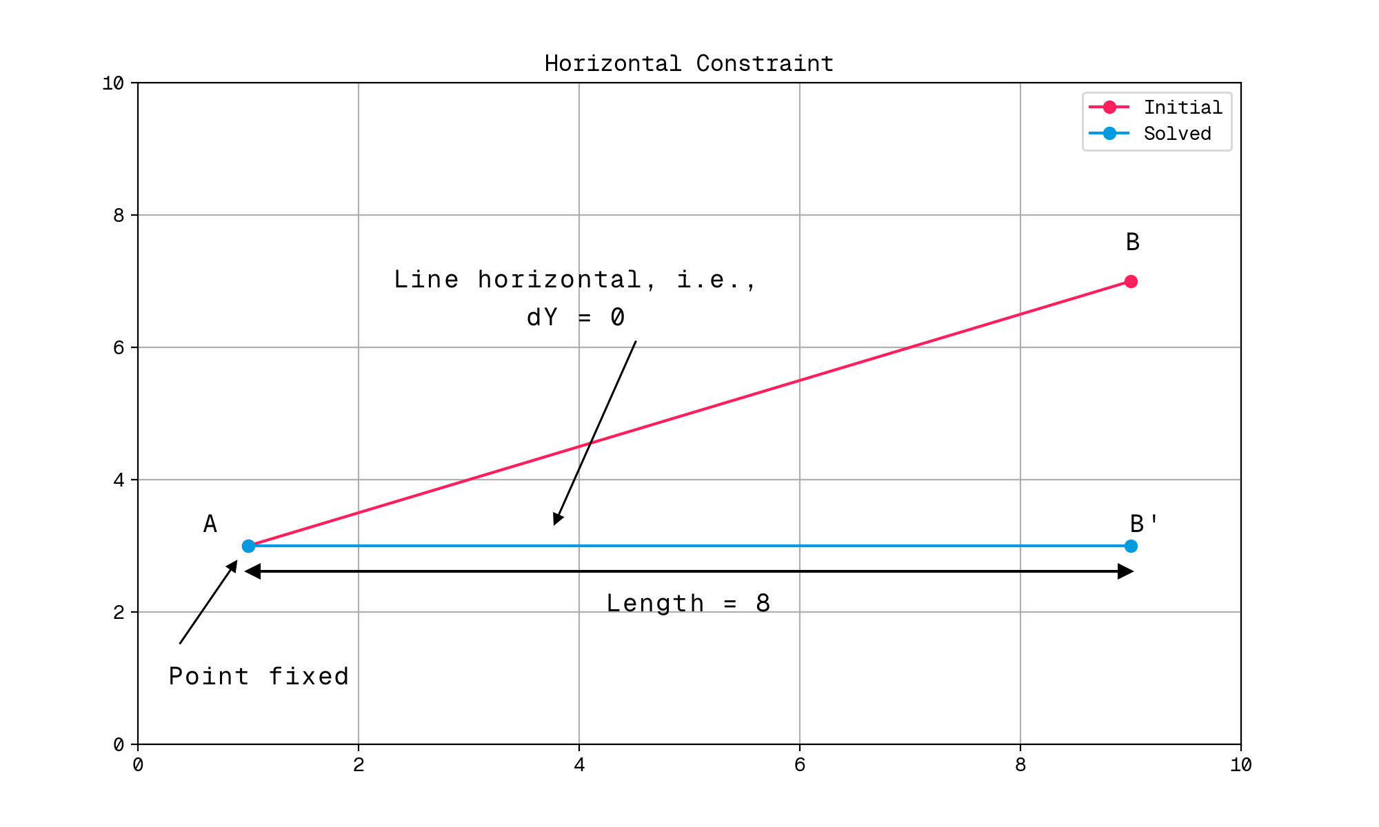
In our case, our constraints are going to be slightly different in nature. In general, we won’t be constraining things like angles or orientations directly, generally defining fixed distances between points instead. However, the principle is the same; we just assemble our residual functions, then use a root-finding algorithm to solve them.

Enter nonlinearity

If you can remember high school level linear algebra, the expression above might look somewhat familiar. Our system was described by:

$$F(x)=r$$

Which is very similar to the standard way of presenting a system of equations in matrix form:

$$Ax=b$$

For now, we’ll focus on the root-finding case, where $r=0$. So, providing our equations are linear and our system, $A$, is square and invertible (so that we can compute a real inverse), we could solve this directly. In terms of actually solving for $x$, there end up being two cases which, for linear systems, are easy to deal with:

• If $b=0$, technically any solution in the null space of $A$ is valid, but $x=0$ is always a valid solution.
• If $b\neq0$ and $A$ is invertible, then a unique solution is given by $x = A^{-1}b$

Moving away from the linear case, to find the roots of our real and nonlinear system, we have to introduce iteration. This brings us into the territory of Newton’s method, which broadly takes the nonlinear $F(x)$, uses the Jacobian (the matrix of first-order derivatives) as a local linear approximation of the system, then solves that approximation to establish a step which we can take towards what are hopefully the actual roots of the system.

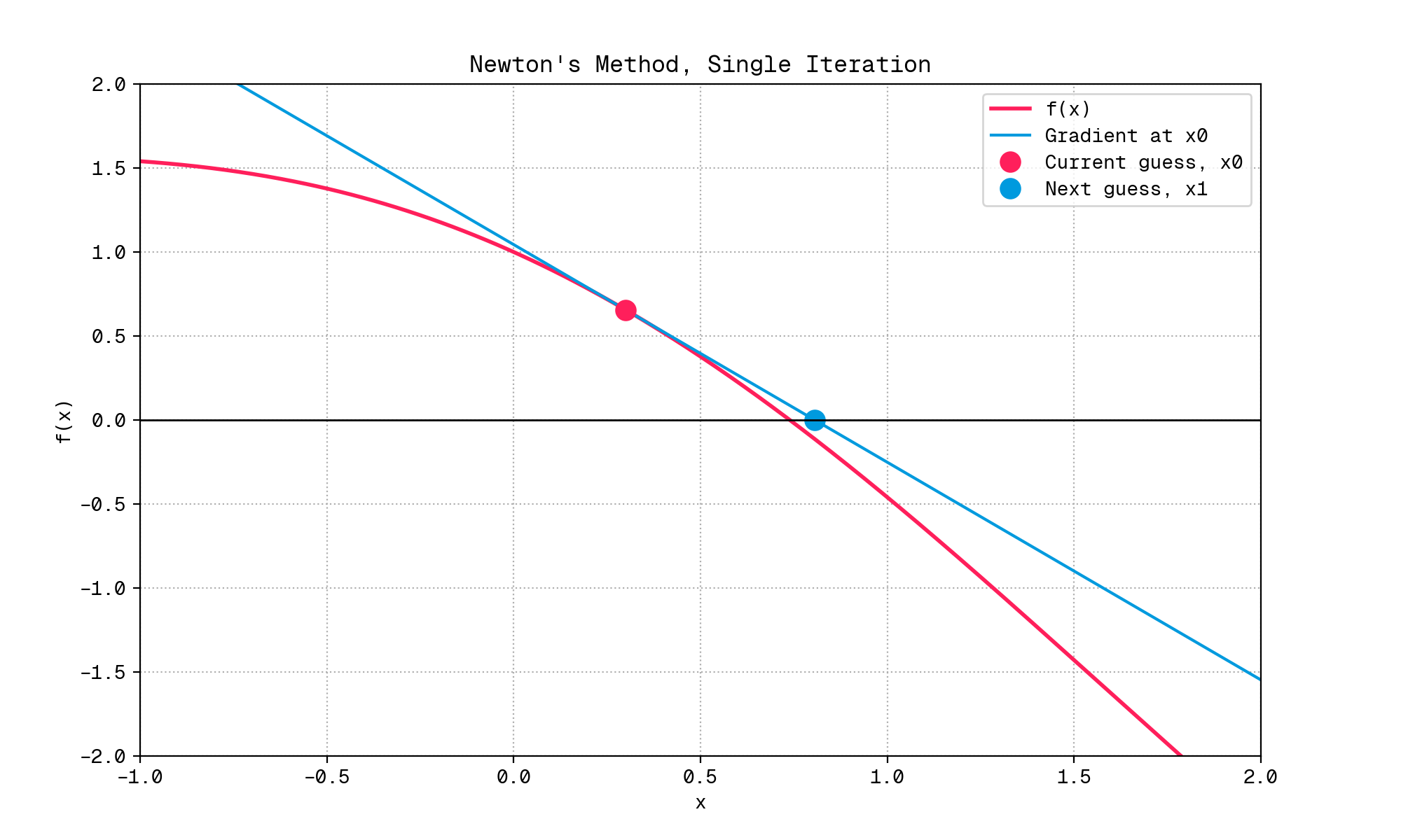
The plot below gives a 1D representation of what we’re actually doing. At a given value of $x$, we can approximate the system by its gradient, and then work out where that intersects our x-axis. If plugging that $x$ back into our real system gives us an answer close to zero, we call this set of $x$ values $x^*$ and consider the system solved. If it doesn’t, we update our $x$ value, recompute our gradient, and solve the new system approximation to find another $x$ step. We then just repeat this process until we converge on the nonlinear system’s actual roots.

At iteration $k$, we take a first-order Taylor expansion of $F$ about $x_k$:

$$ F(x_k + \Delta x_k) \approx F(x_k) + J(x_k) \Delta x_k $$

Where:

• $J(x_{k})$ is the Jacobian at the current guess, $\left[\frac{\partial F_i}{\partial x_j}\right]_{i,j}$.
• $\Delta x_k$ is the step we want to take.

In our case, since we’re trying to find the roots of the system, we want this to be equal to zero.

$$ F(x_{k}) + J(x_{k}) \Delta x_k \approx 0 $$

This is now a linear solve which we can rearrange to be structurally equivalent to our $Ax=b$ case:

$$ J(x_{k}) \Delta x_k = -F(x_{k}) $$

Where:

• $A \equiv J(x_{k})$
• $x \equiv \Delta x_k$
• $b \equiv -F(x_{k})$

Once we solve directly for $\Delta x_k$ using any of the standard methods for solving linear systems, e.g., via LU decomposition, we update our guess for $x$:

$$ x_{k+1} = x_{k} + \Delta x_k $$

We then evaluate $F(x_{k+1})$ with the true nonlinear system to see how close we are to zero, and repeat until convergence.

Rough requirements

Death by math complete, how do we actually build some software to do this for us?

Well, a very simple case isn’t too difficult. We just need to define our residual functions, then pass them to a root-finding algorithm. If we’re willing to use a quasi-Newton method or can bake in automatic differentiation, we can even avoid having to compute the Jacobian ourselves.

Simple example

For example, using fsolve, our 2D horizontal line example from above could be implemented as simply as this:

import numpy as np
from scipy.optimize import fsolve


def point_x_residual(x_actual, x_target):
    return x_actual - x_target


def point_y_residual(y_actual, y_target):
    return y_actual - y_target


def horizontal_line_residual(y_a, y_b):
    return y_b - y_a


def line_length_residual(x_a, y_a, x_b, y_b, target_length):
    current_length = np.sqrt((x_b - x_a) ** 2 + (y_b - y_a) ** 2)
    return target_length - current_length


def build_residuals(variables, target_point_a, target_length):
    x_a, y_a, x_b, y_b = variables

    residuals = [
        point_x_residual(x_a, target_point_a[0]),
        point_y_residual(y_a, target_point_a[1]),
        horizontal_line_residual(y_a, y_b),
        line_length_residual(x_a, y_a, x_b, y_b, target_length),
    ]

    return residuals


if __name__ == "__main__":
    target_point_a = [1.0, 3.0]
    target_length = 8.0

    def residual_func(variables):
        return build_residuals(variables, target_point_a, target_length)

    initial_guess = [0.0, 0.0, 5.0, 5.0]
    solution = fsolve(residual_func, initial_guess, full_output=True)
    variables, info, success, message = solution

    if success == 1:
        x_a, y_a, x_b, y_b = variables
        result = {
            "success": True,
            "point_a": np.array([x_a, y_a]),
            "point_b": np.array([x_b, y_b]),
            "residuals": residual_func(variables),
            "iterations": info["nfev"],
            "message": message,
        }

        print(result)

In practical terms, build_residuals is equivalent to our vector of residual functions, $F(x)$. The variables argument is our current guess vector $x$, and the returned vector of residuals is our $r$. Since we need some of our target information to compute the residuals, we end up a little polluted relative to the maths, but I hope the intent is clear.

When we run it, that produces something like this:

{
  'success': True,
  'point_a': array([1., 3.]),
  'point_b': array([9.,  3.]),
  'residuals': [
    np.float64(0.0),
    np.float64(0.0),
    np.float64(0.0),
    np.float64(0.0)
    ],
  'iterations': 11,
  'message': 'The solution converged.'
}

Under the hood, fsolve is using an estimation of the Jacobian to solve the system; it’s transparently computing a numerical gradient, which costs both performance, in the form of more function evaluations, and accuracy, in the form of approximation error. However, for a simple system like this, it shows how our implementation can be very straightforward.

A little more we might need

In a real-world scenario, most of our heavy lifting will really relate to:

1. Defining a neat method for describing our suspension geometry.
2. Establishing the correct set of constraint/residual functions required by our system.
3. Establishing how best to use those constraints to describe the actual kinematic behaviour of the system.
4. Figuring out how to drive the system, i.e., which variables we want to be able to set directly, and whether we can vary more than one at a time.
5. Providing some mechanism for computing ‘derived’ point positions for points which do not actually influence system kinematics, e.g., wheel centre.
   • If we wish to drive the system based on these derived points, we’ll also need to work out how to express them in terms of the actual hard points, and use that to drive our residuals.

Once we have all of that ironed out, then we can think about whether we need a real Jacobian or not, what exact algorithm to use, how to handle convergence issues, and so on.

In some respects, the core of the problem is quite forgiving. While we might want to accommodate things like redundant links for some more esoteric suspension designs, the classic double wishbone setup should be well determined and consistent, and thus remain a root-finding problem. Having previously sketched out things like a 2D geometric constraint solver for a CAD system, that isn’t always the case, and the maths in this world can sometimes get quite hairy. Thankfully, we shouldn’t have to stress too much about regularisation, condition numbers, least-squares solutions, and so on… at least for now.

Introducing open-kinematics

All of the work on this project has been ironed out in Python, and I’ve pulled together various exploratory bits and pieces into a package called open-kinematics, which is very much a work in progress.

Project basics

I mentioned above how prior experiments with JAX had left me thinking I’d misjudged the best way to achieve something like this with automatic differentiation. As a result, this package does not use automatic differentiation at all; it’s a ’traditional’ solve, which I think of as working from left to right.

The broad flow is:

1. Define the suspension geometry, i.e., hard points, setup etc.
2. Define a ‘sweep’, i.e., a range of wheel centre Z heights or rack positions we want to explore.
3. Ingest that geometry and the sweep data.
4. For each step in the sweep, build and solve the system of equations required to establish the positions of all the points in the system, satisfying the sweep conditions at that step.
5. Compute any metrics of interest, e.g., camber, toe, track, etc.
6. Output the results for the user.

Project structure

This is quite likely to change, particularly as I address some of the shortcomings. However, the project structure is currently something like this:

.
├── justfile
├── LICENSE
├── plot.png
├── PROVENANCE.md
├── pyproject.toml
├── README.md
├── src
│   ├── kinematics
│   │   ├── __init__.py
│   │   ├── cli.py
│   │   ├── constants.py
│   │   ├── constraints.py
│   │   ├── enums.py
│   │   ├── io
│   │   │   ├── geometry_loader.py
│   │   │   ├── results_writer.py
│   │   │   └── sweep_loader.py
│   │   ├── main.py
│   │   ├── metrics
│   │   │   ├── __init__.py
│   │   │   ├── angles.py
│   │   │   ├── antis.py
│   │   │   └── main.py
│   │   ├── points
│   │   │   ├── __init__.py
│   │   │   └── derived
│   │   │       ├── __init__.py
│   │   │       ├── definitions.py
│   │   │       └── manager.py
│   │   ├── solver.py
│   │   ├── state.py
│   │   ├── suspensions
│   │   │   ├── __init__.py
│   │   │   ├── core
│   │   │   │   ├── __init__.py
│   │   │   │   ├── collections.py
│   │   │   │   ├── geometry.py
│   │   │   │   ├── provider.py
│   │   │   │   └── settings.py
│   │   │   ├── implementations
│   │   │   │   ├── __init__.py
│   │   │   │   ├── double_wishbone.py
│   │   │   │   └── macpherson.py
│   │   │   └── registry.py
│   │   ├── targets.py
│   │   ├── types.py
│   │   ├── vector_utils
│   │   │   ├── __init__.py
│   │   │   ├── generic.py
│   │   │   ├── geometric.py
│   │   │   └── visualization.py
│   │   └── visualization
│   │       ├── __init__.py
│   │       ├── animation.py
│   │       ├── api.py
│   │       ├── main.py
│   │       └── plots.py

Key components include:

• src/kinematics/io: Utilities for reading and writing geometry, sweep, and results data.
• src/kinematics/suspensions: Suspension definitions, including points, point collections (e.g., the set of three points that describes a wishbone), and geometry-specific logic.
• src/kinematics/constraints.py: A range of constraint classes, each with a residual() method that computes the residual for that constraint.
• src/kinematics/points: Definitions and management of hard and derived points, where derived points are those whose positions are computed from other points.
• src/kinematics/metrics: Functions for calculating metrics of interest for the solved geometry, e.g., camber, toe, antis, etc.
• src/kinematics/solver.py: The core solver logic, which assembles the system of equations and invokes the root-finding algorithm.

Geometry definition

Geometries are currently defined in YAML files. An example double wishbone geometry is shown below:

type: "DOUBLE_WISHBONE"
name: "test"
version: "0.0.1"
units: "MILLIMETERS"

hard_points:
  lower_wishbone:
    inboard_front:
      x: 250
      y: 400
      z: 200
    inboard_rear:
      x: -250
      y: 450
      z: 200
    outboard:
      x: 0
      y: 900
      z: 200
  upper_wishbone:
    inboard_front:
      x: 225
      y: 350
      z: 500
    inboard_rear:
      x: -275
      y: 350
      z: 500
    outboard:
      x: -25
      y: 750
      z: 500
  wheel_axle:
    # Axle outer point is the hub face.
    inner:
      x: -20
      y: 800
      z: 316.6
    outer:
      x: -20
      y: 950
      z: 313.535
  track_rod:
    inner:
      x: 50
      y: 200
      z: 250
    outer:
      x: 150
      y: 800
      z: 300
configuration:
  steered: true
  wheel:
    offset: 0
    tire:
      aspect_ratio: 0.55
      section_width: 270
      rim_diameter: 13 # SPECIFIED IN INCHES.
  cg_position:
    x: 1250
    y: 0
    z: 450
  wheelbase: 2500.0

The geometry file is largely composed of ‘design condition’ hard point locations, but also includes some configuration data, e.g., whether the system is steered, and some vehicle-level data, e.g., CG position and wheelbase, which we might want to use when computing metrics.

Residual functions

Each concrete class in the constraints module represents a single geometric constraint and contains a residual() method.

As we worked through above, the residual is just an error term; it tells us how much a constraint is being violated. For example, a DistanceConstraint ensures that two points remain a fixed distance apart. Its residual function calculates the current distance between the points and subtracts the target distance:

residual = current_distance - target_distance

When all constraints are met, all residuals are zero. The solver’s entire job is to find the set of 3D coordinates for all the points in the system that satisfies this condition. A range of constraints are required to fully define a suspension system, e.g., distance constraints, angle constraints, point-on-line constraints, and so on.

Here’s a simple example of what these constraint classes look like:

class DistanceConstraint(Constraint):
    """
    Constrains the Euclidean distance between two points.

    This constraint enforces that the distance between two specified points remains
    constant at a target value, useful for rigid links or fixed separations in the
    suspension geometry.
    """

    def __init__(self, p1: PointID, p2: PointID, target_distance: float):
        """
        Initialize the distance constraint.

        Args:
            p1: First point identifier.
            p2: Second point identifier.
            target_distance: The required distance between the points.

        Raises:
            ValueError: If target_distance is negative.
        """
        if target_distance < 0:
            raise ValueError(
                f"Target distance must be non-negative, got {target_distance}"
            )

        self.p1 = p1
        self.p2 = p2
        self.target_distance = target_distance

    @property
    def involved_points(self) -> Set[PointID]:
        return {self.p1, self.p2}

    def residual(self, positions: dict[PointID, Vec3]) -> float:
        """
        Compute the distance residual.

        Returns the difference between the current distance and target distance.
        Positive values indicate the points are too far apart.
        """
        current_distance = compute_point_point_distance(
            positions[self.p1], positions[self.p2]
        )
        return float(current_distance - self.target_distance)

Derived points and DSA

Not all points in a suspension system are really first-class citizens. Many points that we’re interested in have their positions dictated entirely by others; they are not directly constrained by joints or linkages, and do not themselves influence the motion of the system. For example, if we care about an imaginary point at the centre of the wheel, in the wheel’s centre plane, that point is really dictated entirely by the stub axle and the wheel’s offset. That point has no bearing on the system’s kinematics; but we do care about it, and may want to ‘drive’ the system by setting its position to some target value and then solving for where everything else needs to be to achieve that.

In this system’s nomenclature, we refer to these ‘imaginary’ points as derived points; they are derived from the hard points that actually define the system’s behaviour. From the outset, I wanted the system to support the concept of derived points which are themselves derived from other derived points. If, to wring the life out of the stub axle example, we define our axle with inboard and outboard points, then define our wheel centre from those, then decide we want to know about a point 30mm inboard of the wheel centre, we could define that point as being derived, in part, from the wheel centre, which is itself derived from the stub axle points.

To handle this, the DerivedPointsManager class represents the dependencies between derived points as a directed acyclic graph (DAG). In this graph, each node corresponds to a point ID, and each edge represents a dependency where one point’s position relies on another. For example, if point A depends on point B, there’s an edge from A to B. We enforce that this graph remains acyclic through depth-first search (DFS) cycle detection, preventing circular dependencies where a point might transitively depend on itself. However, the actual appeal of this approach comes when we perform a topological sort of the graph. This sort allows us to assemble a list of points in an order such that any point appears after all the points it depends on, enabling us to calculate all derived points in a single pass with the guarantee that all dependencies are already computed.

During the solve, after the solver makes a guess for the free points, the manager simply iterates through this pre-sorted list, calculating each derived point in the correct sequence. This ensures that when the residual functions are evaluated, they have access to a complete and consistent set of coordinates for the entire system.

The actual manager class looks something like this:

class DerivedPointsManager:
    """
    Manages the calculation of derived points by building and resolving a dependency
    graph to ensure the correct update order.
    """

    def __init__(self, spec: DerivedPointsSpec):
        self.spec = spec
        self.dependency_graph = spec.dependencies

        # This will raise an error if cycles are detected.
        self.update_order = self.get_topological_sort()

    def detect_cycles_util(
        self, node: PointID, visited: set, recursion_stack: set
    ) -> bool:
        """
        Depth-first search utility for cycle detection in dependency graph.

        Uses two sets to track node states during DFS traversal:
        - visited: nodes that have been completely processed
        - recursion_stack: nodes in the current DFS path being explored

        A cycle is detected when we encounter a node that's already in the
        current recursion stack, indicating a back edge.

        Args:
            node: Current node being explored in the dependency graph.
            visited: Set of nodes that have been completely processed.
            recursion_stack: Set of nodes in the current DFS path.

        Returns:
            True if a cycle is detected starting from this node, False otherwise.
        """
        visited.add(node)
        recursion_stack.add(node)

        for neighbor in self.dependency_graph.get(node, set()):
            if neighbor not in visited:
                if self.detect_cycles_util(neighbor, visited, recursion_stack):
                    return True
            elif neighbor in recursion_stack:
                return True  # Cycle detected

        recursion_stack.remove(node)
        return False

    def get_topological_sort(self) -> list[PointID]:
        """
        Performs a topological sort of the derived points to determine the correct
        calculation order.

        Raises:
            ValueError: If a circular dependency is detected in the graph.
        """
        visited = set()
        recursion_stack = set()
        nodes = set(self.dependency_graph.keys())

        for node in nodes:
            if node not in visited:
                if self.detect_cycles_util(node, visited, recursion_stack):
                    raise ValueError(
                        "Circular dependency detected in derived point definitions."
                    )

        visited.clear()
        order = []

        def dfs(node: PointID):
            if node in visited:
                return
            visited.add(node)

            # Recurse on dependencies that are also derived points
            for dep in self.dependency_graph.get(node, set()):
                if dep in self.spec.functions:
                    dfs(dep)

            order.append(node)

        for point_id in self.spec.functions:
            if point_id not in visited:
                dfs(point_id)

        return order

    def update_in_place(self, positions: dict[PointID, Vec3]) -> None:
        """
        Compute derived points and add them to positions dict in-place.

        Args:
            positions: Dictionary to mutate in-place by adding derived points.
        """
        for point_id in self.update_order:
            update_func = self.spec.functions[point_id]
            positions[point_id] = update_func(positions)

The DoubleWishboneProvider

In the suspensions/implementations module, we have concrete implementations of the suspension types we want to support. For each type, we centralise the geometry-specific logic, primarily for the benefit of developer experience.

For example, for a double wishbone layout, we have the DoubleWishboneProvider class, which provides functionality to read the geometry, create an initial state, define which points are free to move, specify how derived points are computed, and declare the constraints required to fully define the system.

It is also where we will provide geometry-specific visualisation information and metric calculation tools, e.g., for computing instant centres, given that the approach requried here varies between suspension types.

class DoubleWishboneProvider(SuspensionProvider):
    """
    Concrete implementation of SuspensionProvider for double wishbone geometry.
    """

    def __init__(self, geometry: DoubleWishboneGeometry):
        """
        Initialize the double wishbone provider.

        Args:
            geometry: Double wishbone geometry configuration.
        """
        self.geometry = geometry

    def initial_state(self) -> SuspensionState:
        """
        Create initial suspension state from geometry hard points.

        Converts the hard point coordinates from the geometry into a SuspensionState
        with both explicitly defined and derived points.

        Returns:
            Initial suspension state with all point positions.
        """
        positions = {}
        hard_points = self.geometry.hard_points

        # Lower wishbone.
        lwb = hard_points.lower_wishbone
        positions[PointID.LOWER_WISHBONE_INBOARD_FRONT] = np.array(
            [lwb.inboard_front["x"], lwb.inboard_front["y"], lwb.inboard_front["z"]]
        )
        positions[PointID.LOWER_WISHBONE_INBOARD_REAR] = np.array(
            [lwb.inboard_rear["x"], lwb.inboard_rear["y"], lwb.inboard_rear["z"]]
        )
        positions[PointID.LOWER_WISHBONE_OUTBOARD] = np.array(
            [lwb.outboard["x"], lwb.outboard["y"], lwb.outboard["z"]]
        )

        # Upper wishbone.
        uwb = hard_points.upper_wishbone
        positions[PointID.UPPER_WISHBONE_INBOARD_FRONT] = np.array(
            [uwb.inboard_front["x"], uwb.inboard_front["y"], uwb.inboard_front["z"]]
        )
        positions[PointID.UPPER_WISHBONE_INBOARD_REAR] = np.array(
            [uwb.inboard_rear["x"], uwb.inboard_rear["y"], uwb.inboard_rear["z"]]
        )
        positions[PointID.UPPER_WISHBONE_OUTBOARD] = np.array(
            [uwb.outboard["x"], uwb.outboard["y"], uwb.outboard["z"]]
        )

        # Track rod.
        tr = hard_points.track_rod
        positions[PointID.TRACKROD_INBOARD] = np.array(
            [tr.inner["x"], tr.inner["y"], tr.inner["z"]]
        )
        positions[PointID.TRACKROD_OUTBOARD] = np.array(
            [tr.outer["x"], tr.outer["y"], tr.outer["z"]]
        )

        # Wheel axle
        wa = hard_points.wheel_axle
        positions[PointID.AXLE_INBOARD] = np.array(
            [wa.inner["x"], wa.inner["y"], wa.inner["z"]]
        )
        positions[PointID.AXLE_OUTBOARD] = np.array(
            [wa.outer["x"], wa.outer["y"], wa.outer["z"]]
        )

        # Calculate derived points to create a complete initial state.
        derived_spec = self.derived_spec()
        derived_resolver = DerivedPointsManager(derived_spec)
        derived_resolver.update_in_place(positions)

        return SuspensionState(positions=positions, free_points=set(self.free_points()))

    def free_points(self) -> Sequence[PointID]:
        """
        Define which points the solver can move during optimization.

        Returns:
            Sequence of point IDs that are free to move (outboard and axle points).
        """
        return [
            PointID.UPPER_WISHBONE_OUTBOARD,
            PointID.LOWER_WISHBONE_OUTBOARD,
            PointID.AXLE_INBOARD,
            PointID.AXLE_OUTBOARD,
            PointID.TRACKROD_OUTBOARD,
            PointID.TRACKROD_INBOARD,
        ]

    def derived_spec(self) -> DerivedPointsSpec:
        """
        Define specifications for computing derived points from free points.

        Returns:
            Specification containing functions and dependencies for derived points.
        """
        wheel_cfg = self.geometry.configuration.wheel
        # Use the nominal tire radius from the configuration.
        tire_radius = self.geometry.configuration.wheel.tire.nominal_radius

        functions = {
            PointID.AXLE_MIDPOINT: get_axle_midpoint,
            PointID.WHEEL_CENTER: partial(
                get_wheel_center, wheel_offset=wheel_cfg.offset
            ),
            PointID.WHEEL_INBOARD: partial(
                get_wheel_inboard, wheel_width=wheel_cfg.tire.section_width
            ),
            PointID.WHEEL_OUTBOARD: partial(
                get_wheel_outboard, wheel_width=wheel_cfg.tire.section_width
            ),
            PointID.WHEEL_CENTER_ON_GROUND: partial(get_wheel_center_on_ground),
            PointID.CONTACT_PATCH_CENTER: partial(
                get_contact_patch_center, tire_radius=tire_radius
            ),
        }

        dependencies = {
            PointID.AXLE_MIDPOINT: {PointID.AXLE_INBOARD, PointID.AXLE_OUTBOARD},
            PointID.WHEEL_CENTER: {PointID.AXLE_INBOARD, PointID.AXLE_OUTBOARD},
            PointID.WHEEL_INBOARD: {PointID.WHEEL_CENTER, PointID.AXLE_INBOARD},
            PointID.WHEEL_OUTBOARD: {PointID.WHEEL_CENTER, PointID.AXLE_INBOARD},
            PointID.WHEEL_CENTER_ON_GROUND: {
                PointID.WHEEL_CENTER,
                PointID.AXLE_INBOARD,
                PointID.AXLE_OUTBOARD,
            },
            PointID.CONTACT_PATCH_CENTER: {
                PointID.WHEEL_CENTER,
                PointID.AXLE_INBOARD,
                PointID.AXLE_OUTBOARD,
            },
        }

        return DerivedPointsSpec(functions=functions, dependencies=dependencies)

    def constraints(self) -> list[Constraint]:
        """
        Build the complete set of geometric constraints for double wishbone suspension.

        Returns:
            List of constraints that must be satisfied during kinematic solving.
        """
        constraints: list[Constraint] = []
        initial_state = self.initial_state()

        # Distance constraints.
        length_pairs = [
            (PointID.UPPER_WISHBONE_INBOARD_FRONT, PointID.UPPER_WISHBONE_OUTBOARD),
            (PointID.UPPER_WISHBONE_INBOARD_REAR, PointID.UPPER_WISHBONE_OUTBOARD),
            (PointID.LOWER_WISHBONE_INBOARD_FRONT, PointID.LOWER_WISHBONE_OUTBOARD),
            (PointID.LOWER_WISHBONE_INBOARD_REAR, PointID.LOWER_WISHBONE_OUTBOARD),
            (PointID.UPPER_WISHBONE_OUTBOARD, PointID.LOWER_WISHBONE_OUTBOARD),
            (PointID.AXLE_INBOARD, PointID.AXLE_OUTBOARD),
            (PointID.AXLE_INBOARD, PointID.UPPER_WISHBONE_OUTBOARD),
            (PointID.AXLE_INBOARD, PointID.LOWER_WISHBONE_OUTBOARD),
            (PointID.AXLE_OUTBOARD, PointID.UPPER_WISHBONE_OUTBOARD),
            (PointID.AXLE_OUTBOARD, PointID.LOWER_WISHBONE_OUTBOARD),
            (PointID.TRACKROD_INBOARD, PointID.TRACKROD_OUTBOARD),
            (PointID.UPPER_WISHBONE_OUTBOARD, PointID.TRACKROD_OUTBOARD),
            (PointID.LOWER_WISHBONE_OUTBOARD, PointID.TRACKROD_OUTBOARD),
            (PointID.AXLE_INBOARD, PointID.TRACKROD_OUTBOARD),
            (PointID.AXLE_OUTBOARD, PointID.TRACKROD_OUTBOARD),
        ]
        for p1, p2 in length_pairs:
            target_distance = compute_point_point_distance(
                initial_state.positions[p1], initial_state.positions[p2]
            )
            constraints.append(DistanceConstraint(p1, p2, target_distance))

        # Angle constraints.
        v1 = make_vec3(
            initial_state.positions[PointID.LOWER_WISHBONE_OUTBOARD]
            - initial_state.positions[PointID.UPPER_WISHBONE_OUTBOARD]
        )
        v2 = make_vec3(
            initial_state.positions[PointID.AXLE_OUTBOARD]
            - initial_state.positions[PointID.AXLE_INBOARD]
        )
        target_angle = compute_vector_vector_angle(v1, v2)

        constraints.append(
            AngleConstraint(
                v1_start=PointID.UPPER_WISHBONE_OUTBOARD,
                v1_end=PointID.LOWER_WISHBONE_OUTBOARD,
                v2_start=PointID.AXLE_INBOARD,
                v2_end=PointID.AXLE_OUTBOARD,
                target_angle=target_angle,
            )
        )

        # Point-on-line constraints.
        constraints.append(
            PointOnLineConstraint(
                point_id=PointID.TRACKROD_INBOARD,
                line_point=initial_state.positions[PointID.TRACKROD_INBOARD],
                line_direction=WorldAxisSystem.Y,
            )
        )

        return constraints

Solver specifics

With our constraints defined and a mechanism for the reliable calculation of all derived point positions, plus appropriate code for gluing all of this logic together, we can finally get to actually solving. The main logic resides in src/kinematics/solver.py.

For each step of a sweep (e.g., a specific wheel centre Z-height), the solver is tasked with finding the roots of system of nonlinear equations. More directly, that just means we need to find the set of free point coordinates (x, y, z) that makes the vector of all residual values equal to zero.

On solver methods

Above, we discussed the general approach of using Newton’s method for root finding. Pure Newton’s method should work perfectly well for this sort of problem, but comes with two important practical requirements:

1. We would need to compute the Jacobian matrix for our system.
2. Our system of equations would have to be square and of full rank.

That first point isn’t too bad; we can throw sympy at the problem or even just grind those derivatives out by hand. However, the second point is more problematic. While I think most well-defined suspension systems are likely to meet these conditions, I don’t think we can guarantee that they always will. For example, if we have any redundant links, that will introduce extra constraints and render the system overdetermined and thus non-square, even if those constraints are consistent. Equally, if we are at all careless with our constraint setup and our constraint definitions happen to introduce some redundancy, despite not contradicting the system’s actual geometry, we could end up with a system that is not soluble with pure Newton’s method.

As we move away from the textbook cases here, we can start to look at approaches which expand on Newton’s method, while still following the same broad principle of iteratively solving a linear approximation of the nonlinear system.

In my day job at Zoo, I approached a similar problem by adopting explicit Tikhonov regularisation to handle underdetermined systems, and patched in a QR decomposition method in lieu of a direct LU factorisation for a least squares version of the inner linear solve; see this and this. This approach worked well, given that we needed to accommodate both underdetermined and overdetermined systems and needed to work out how to get a solver running in Rust… but in this case, we can just go ‘shopping’ for a ready-made solver in SciPy.

In terms of what we actually want to ‘buy’ here, we’re looking for something that we can use for multivariate nonlinear root finding, which can handle non-square systems, and which is reasonably robust. By virtue of needing to support non-square systems, we’re really looking for a least-squares approach, which means we can rule out pure Newton’s method.

Basically, instead of solving for $F(x) = 0$ directly (which we can’t do because we’d need a square matrix), we try to solve for $||F(x)||^2 = 0$, which we can do. When this least squares condition is met, helpfully, it means that $F(x) = 0$ as well.

Thankfully, SciPy provides a few options we could use. The most obvious, and the one I’ve adopted, is Levenberg-Marquardt. It’s a little bit like a fancy version of the Zoo Tikhonov regularisation and QR inner solve approach; it is damped, similar to the effect we introduced with Tikhonov regularisation, but the damping is adaptive. Instead of having a fixed regularisation term, it adjusts the damping factor based on how well the last step performed, essentially blending between Gauss-Newton and gradient descent. This adaptive damping helps to ensure that the solve remains stable and converges reliably, even when the initial guess is far from the solution.

Being lazy with the Jacobian

Our Levenberg-Marquardt implementation, via SciPy’s least_squares function, lets us be somewhat lazy, at least to start. If we don’t pass a function to compute the Jacobian, it will default to performing a finite difference approximation. This is not ideal; it means we have to call our residual functions multiple times per iteration to estimate the gradient, which is both slower and less accurate than an analytical Jacobian. However, it allows us to exercise the rest of the system without having to trouble sympy.

In practice

With the finite difference Jacobian approximation, the actual solve call, in the context of a sweep, looks like this:

def solve_suspension_sweep(
    initial_state: SuspensionState,
    constraints: list[Constraint],
    sweep_config: SweepConfig,
    derived_manager: DerivedPointsManager,
    solver_config: SolverConfig = SolverConfig(),
) -> tuple[list[SuspensionState], list[SolverInfo]]:
    """
    Solves a series of kinematic states by sweeping through target configurations using
    damped non-linear least squares. This function performs a sweep where each step in
    the sweep corresponds to a set of targets, solving sequentially from the initial
    state. All state and residual buffers are reused across evaluations to minimize
    allocations.

    Args:
        initial_state (SuspensionState): The initial suspension state to start the sweep from.
        constraints (list[Constraint]): List of geometric constraints to satisfy.
        sweep_config (SweepConfig): Configuration for the sweep, including number of steps and target sweeps.
        derived_manager (DerivedPointsManager): Manager to compute derived points in-place.
        solver_config (SolverConfig): Configuration parameters for the solver.

    Returns:
        Tuple of (solved_states, solver_stats) where:
        - solved_states: List of converged suspension states for each sweep step
        - solver_stats: List of solver diagnostics for each step

    Raises:
        ValueError: If the system is underdetermined (more variables than residuals).
        RuntimeError: If the solver fails to converge at any step.
    """
    # Convert all targets to absolute coordinates once before solving.
    sweep_targets = [
        convert_targets_to_absolute(
            [sweep[i] for sweep in sweep_config.target_sweeps], initial_state
        )
        for i in range(sweep_config.n_steps)
    ]

    # Working state reused across the sweep; mutated in-place for performance.
    working_state = initial_state.copy()

    # For each step in our sweep, we will keep a copy of the solved state; this is
    # our result dataset.
    solution_states: list[SuspensionState] = []
    solver_stats: list[SolverInfo] = []

    # Create residual computer with pre-allocated buffers.
    # This single instance is reused across all solver evaluations in the sweep.
    residual_computer = ResidualComputer(
        constraints=constraints,
        derived_manager=derived_manager,
        state_buffer=working_state,
        n_target_variables=len(sweep_config.target_sweeps),
    )

    # Initial guess built from the working state's free points.
    x_0 = working_state.get_free_array()

    for step_targets in sweep_targets:
        n_vars = len(working_state.free_points_order) * 3
        m_res = len(constraints) + len(step_targets)

        if n_vars > m_res:
            raise ValueError(
                f"System is underdetermined (n_vars={n_vars} > m_res={m_res}). "
                "The solve method (Levenberg-Marquardt) requires at least as "
                "many residuals as variables."
            )

        result = least_squares(
            fun=residual_computer.compute,
            x0=x_0,
            args=(step_targets,),
            method=SOLVE_METHOD,
            ftol=solver_config.ftol,
            xtol=solver_config.xtol,
            gtol=solver_config.gtol,
            verbose=solver_config.verbose,
        )

        if not result.success:
            raise RuntimeError(
                f"Solver failed to converge for targets: {step_targets}."
                f"\nMessage: {result.message}"
            )

        # We now have to synchronize working_state with the accepted solution.
        # The solver evaluates residuals at many candidate positions during the solve,
        # mutating working_state each time. When it terminates, working_state may be left
        # at a position from gradient estimation (e.g., x* + epsilon) rather than
        # the actual solution x*. We must explicitly restore it to result.x to
        # ensure the stored state matches the returned solution.
        #
        # This synchronization is necessary because we reuse working_state across all
        # residual evaluations for performance (avoiding dict allocations on each call).
        # The tradeoff is this explicit sync requirement.
        working_state.update_from_array(result.x)
        derived_manager.update_in_place(working_state.positions)

        # Store finalized state for this step.
        solution_states.append(working_state.copy())

        # Collect solver information for this step.
        max_residual = float(np.max(np.abs(result.fun))) if len(result.fun) > 0 else 0.0
        solver_info = SolverInfo(
            converged=result.success,
            nfev=result.nfev,
            max_residual=max_residual,
        )
        solver_stats.append(solver_info)

        # The result becomes our local first guess for the next step.
        x_0 = result.x

    return solution_states, solver_stats

CLI tools and visualisation

In the interest of simplicity, I opted for a CLI mechanism to run the solver and output results, and there are currently two commands that are useful.

For a specific geometry, we can visualise the ‘design condition’ as laid out in the geometry file. This command also runs a quick check where corner’s ‘contact patch’ is relative to the ground. (We don’t actually have any variety of tyre model in here, so this is really just telling us whether or not a circle, drawn on the wheel’s centre plane, has its lowest point at Z=0.)

uv run kinematics visualize --geometry=tests/data/geometry.yaml --output=plot.png

Then, if we feed in a sweep definition, we can run that sweep and output the results to a CSV or Parquet file, then assemble an animation of the motion.

uv run kinematics sweep --geometry=tests/data/geometry.yaml --sweep=tests/data/sweep.yaml --out=results.csv --animation-out=anim.mp4

In this example, we’re sweeping both wheel centre Z height and rack position with this sweep configuration:

version: 1
steps: 41
targets:
  - point: TRACKROD_INBOARD
    direction:
      axis: Y
    mode: relative
    start: -40
    stop: 40
  - point: WHEEL_CENTER
    direction:
      axis: Z
    start: -40
    stop: 120

What we didn’t get to

Solving for positions, as shown above, is really just the first step in building a useful tool for real vehicle dynamics bods. We have not addressed the computation of metrics at all, and the body of work required there is pretty substantial. We would need to look at, at least:

• Camber,
• Caster,
• Toe,
• Kingpin inclination,
• Scrub radius,
• FVSA length,
• SVSA length,
• Roll centre,
• Anti-dive,
• Anti-squat.

…plus whatever else I’ve forgotten. Some of these are quite straightforward, others more involved. For example, the computation of antis is likely to push us down the route of needing to compute wishbone plane intersections to arrive at instant axes, which we then convert to instant centres as projected on the relevant principal plane, which we then plug into our anti calc.

We also haven’t built anything to account for adjustability of the system. For example, a typical open-wheel racing car is likely to have readily adjustable camber and toe settings, generally adjusted with shims. It is also extremely likely to have some form of ride height adjustment, which can take a few forms.

Camber, in particular, poses a fun challenge here, as the F1-style camber block arrangement effectively alters the geometry of the upright itself. As shims are added, they induce rotation of the main upright body about the lower balljoint, bringing the stub axle with it, and causing wheel camber to become more positive… all while leaving the upper balljoint position unchanged.

To show what I mean, here’s an image of a 2014 Caterham upright:

If we mark that up to make the important features a little more obvious, you can see how additional shims would really push the upright body outboard at the top, rotating it about the lower balljoint, and thus changing the camber:

Similar arrangements can also be found on less exotic cars, like this assembly for a Lotus Elise:

These are all things we’ll need to account for, even with a simple system, should we want it to be of any use in the real-world.

To be continued…

Links

• See the open-kinematics project on GitHub.