Differentiable programming in engineering
Design, partial derivatives, and the allure of automatic differentiation.
Contents:
Motivation
This post is just intended to serve as a longer form version of my thoughts on differentiable programming in engineering. It’s effectively a follow-up to a lot of back and forth on this Twitter thread, where a whole bunch of us were discussing differentiable programming in engineering. The folks involved were:
- Stellarator engineer, @Andercot,
- Zoo/KittyCAD CEO, @jessfraz,
- Firstname Bunchofnumbers and design automation tinkerer, @Weston212872500,
- Me, @nick_mccleery.
Plus a fleeting contribution from @afshawnl.
Why you might want gradients: Part 1
Before I start into the mechanics of finite differences, analytical derivatives, and automatic differentiation, it’s worth outlining at a very high level why any of this might be useful at all. Within the existing paradigm that we use to design and develop physical systems, and without getting into the inner workings of relevant things I definitely don’t understand, like how OpenFOAM sets about solving the Navier-Stokes equations, there are three standout use cases that I can see.
#1: Sensitivity analysis
The most obvious use case for knowing the rate at which some parameter changes in relation to another, at least to me, is in simple sensitivity analysis. For many systems, we’re often interested in how some parameter will respond to changes in another. You could be interested in how roadwheel camber angle responds to vertical hub displacement, how system pressure responds to a change in temperature, or how much further a beam will deflect if asked to span a longer distance.
For me, the thinking here is basically “what would be the change in y for some nominal change in x?"—effectively $dy/dx$—and it’s the sort of thing you often want to have some broad knowledge of because it provides you with understanding and feel for the system. It doesn’t really matter what these parameters are, or what the system is; it’s just useful to have a feel for how the system will respond to changes in its inputs.
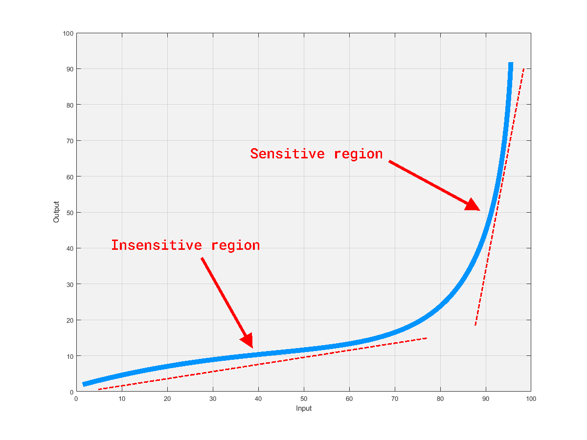
Here’s a very simple example that I would broadly think of as bilinear. This thing has two regimes; one where the output is not very sensitive to change in input, and one where it is. I’d look at this and then commit to memory some simplified notion that the system has a knee point at an input value of about $80$, and that the output is pretty sensitive to changes in input from then on.
Why you might want to have this knowledge of and feel for a system feeds into the next point.
#2: Optimisation
Why optimisation?
Many engineering challenges are effectively optimisation problems. You might want to calibrate your engine to make as much power as possible without it disintegrating, to design a bridge that uses as little material as possible without collapsing, or to pick the right combination of setup options to help your car navigate a circuit as quickly as possible.
In all of these cases, you basically have some objective function that you want to maximise or minimise subject to a set of constraints. The objective function might be incredibly complex because you have to consider a whole list of competing factors. For example, maybe your engine could make more power if you could change the exhaust design, but then you might not be able to package the engine in the full lineup it’s expected to serve,and you want to maintain as many common parts across the range as possible, so this is undesirable.
There’s a lot of this trade-off style decision making that goes into engineering, and this often involves several people, each with different specialities and who each have some feel for the sensitivities of their own particular part of the system. This means the optimisation happens somewhat organically,with conversations and meetings and presentations that eventually yield what’s thought to the best overall compromise for whatever the particular target was.
However, there are some cases where you can do this with a computer. You can write a program that will explore the design space and find the best solution. For example, you might want to determine the aerofoil profile that will give you the minimum amount of drag while your aircraft is in cruise, while still generating enough lift for take-off under hot and high conditions.
In this scenario, you want an optimisation routine that can modify the wing profile, compute the relevant lift and drag forces under the specified conditions, verify that all constraints are met, and then move on to the next iteration,all the time homing in on the best solution.
What does that have to do with gradients?
I have certainly done things like this without having really explicitly calculated any gradients at all. I’ve built
tools that use fminsearch to hunt down the best
compromise solution to some problem by repeatedly calling on some 1D and 2D simulations, bottomed out long running
measurement issues by tasking
Excel’s Solver add-in
to find the best fit correction factor for some data, and I’ve built things that use
Brent’s method across a few programming languages.
Credit: https://commons.wikimedia.org/wiki/User:Nicoguaro
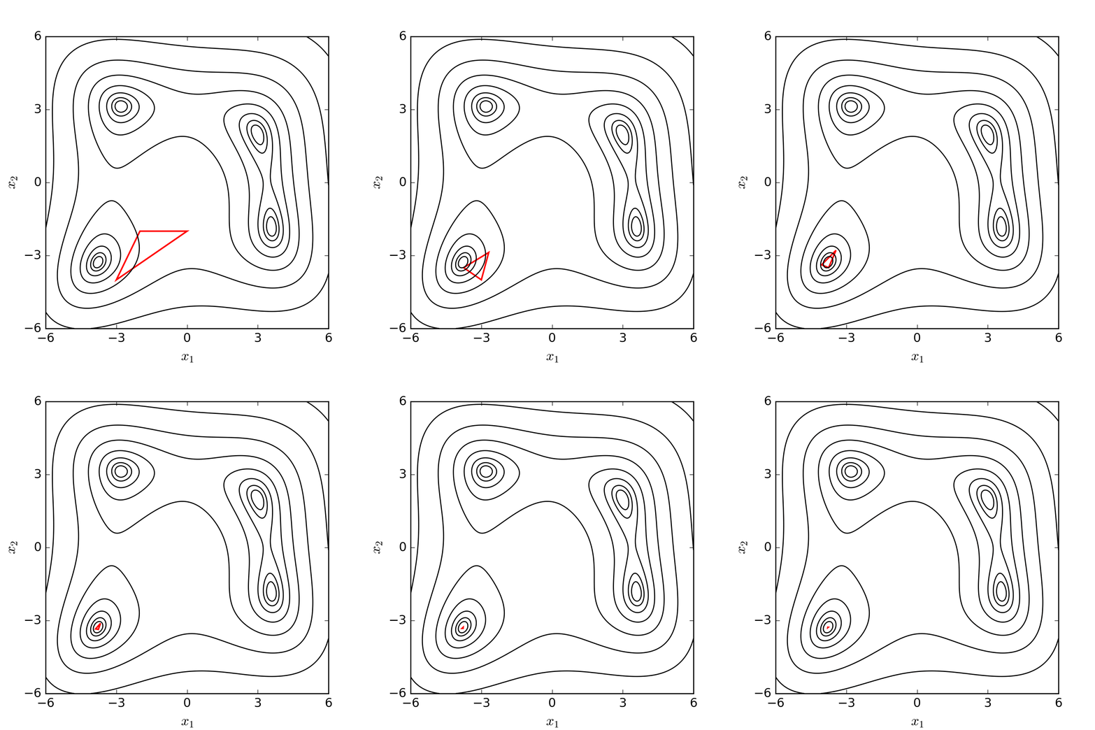
However, in some of these cases, and particuarly where Brent’s method is effectively using the secant method, we are basically doing a finite difference version of Newton’s method, ultimately evaluating our objective function at at least two points, and then using our two output values and our step size to inform our next guess.
At some point, what we are actually doing here is numerically estimating the gradient of our objective function with respect to our design variables. So gradients are actually pretty fundamental to a lot of the optimisation that we do, and this invites some questioning about whether we could do better… which I’ll come back to shortly.
#3: Control systems
The other use case that jumps out at me is control systems. I’m acutely aware that I’ll get out of my depth here quickly, so this should be short and sweet.
Control is about governing the behaviour of dynamic systems such that they do what their designer intended in a regulated, stable, performant manner. That could mean designing a system that controls the amount of torque delivered to the rear wheels of a car in order to help drivers reduce time lost to wheel spin. Or, it could mean designing a system that selectively adjusts engine firing, thruster firing, and control surface position in order to help a rocket reverse itself onto a barge.
To achieve this, you need to know how your system will respond to changes in its inputs, and often the control strategy does too. The more direct use-cases I can think of are:
- Stability analysis.
- Assessing how system stability changes with changes in parameters—particularly so you can suss out stability margin sensitivity to changes in parameters, so you can ensure the system won’t become unstable at some corner of its operating envelope.
- Parameter tuning.
- Adjusting control system parameters to achieve desired system behaviour, often involving a gradient-based optimisation routine. Gradient-based approaches are particularly attractive when you have a complex set of metrics to deal with, as these can help you find optimal settings quickly… and this is a topic we’ll come back to.
- On top of this, the ‘D’ in ‘PID’ stands for ‘derivative’—so where this term is actually set, the control system is using rate of change of the error signal to inform its next move.
- Model predictive control and model reference adaptive control.
- MPC uses gradients to optimise control inputs over some specified future horizon based on a system model, aiming to minimise a cost function that often includes terms for error, control effort, and constraints.
- MRAC adjusts the controller parameters in real-time to match the behavior of the system to a reference model. Gradients in this context are used to update controller parameters to minimise the difference between the actual system behavior and the reference model.
Why you might want gradients: Part 2
Here I want to zoom in on the design optimisation piece. This is the area where I think the potential for differentiable programming is most obvious, and where I think it could have the most impact.
The panacea of design optimisation here is probably something like a flexible, paramaterised CAD model that’s closely coupled with a relevant set of simulation tools—CFD, FEA, MBS, etc.—and an optimisation routine that can explore the design space to find the best overall solution in an acceptably short period of time.
The process for this would ultimately be an iterative one, where you’d start with some initial design, run some simulations, evaluate the results, and then use the results to inform the next iteration of the design,repeating this process until you arrive at some global optimum that forms your final design.
I-beam example
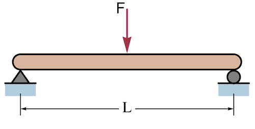
To give an offensively simplified example of the broad process we would want to see here, let’s pretend we have a parametric model of a simply supported, symmetrical I-beam that’s going to carry a central point load. We have the freedom to adjust two of its parameters: overall external depth and overall breadth. Our goal is purely to minimise deflection, and we have the following constraints on our design variables:
- The depth must be between 100mm and 200mm.
- The breadth must be between 50mm and 100mm.
Setup
Here’s the section we’re talking about with our free variables highlighted:
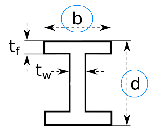
Now, for anyone who’s got the $bd^3/12$ formula etched into their brain, you can see where we’re going to end up here,but let’s pretend we don’t know the answer already.
This is the scenario we’re talking about:
Credit: https://commons.wikimedia.org/wiki/File:Simple_beam_with_center_load.svg
And our equation for deflection at the centre of the beam is: $$ \delta = \frac{F L^3}{48 E I} $$
Where:
- $\delta$ is the deflection at the centre of the beam,
- $F$ is the force applied to the beam,
- $L$ is the length of the beam,
- $E$ is the modulus of elasticity of the beam material,
- $I$ is the second moment of area of the beam’s cross section.
Objective function
We are trying to find the design that would give us the least deflection, so our objective is to minimise $\delta$. We can do that by adjusting the beam section, which directly influences $I$. We will keep load, span, material, and other section properties fixed,using values as follows:
- $F$ = 20kN,
- $L$ = 2000mm,
- $E$ = 200GPa,
- $t_w$, web thickness = 5mm,
- $t_f$, flange thickness = 5mm.
Brute force and ignorance
For a problem like this, it’s not computationally challenging to explore the full design space. We can define a depth series at 1mm increments, a breadth series at 1mm increments, then work through the calculations for $I$ and then $\delta$ at each point.
In this way, we arrive at a nice 2D matrix of deflection values; one for each $(b, d)$ pair. I think this is a fairly nice way to visualise how an engineering problem might be thought of as an optimisation problem; we’re simply trying to find the position on this surface that has the minimum value.
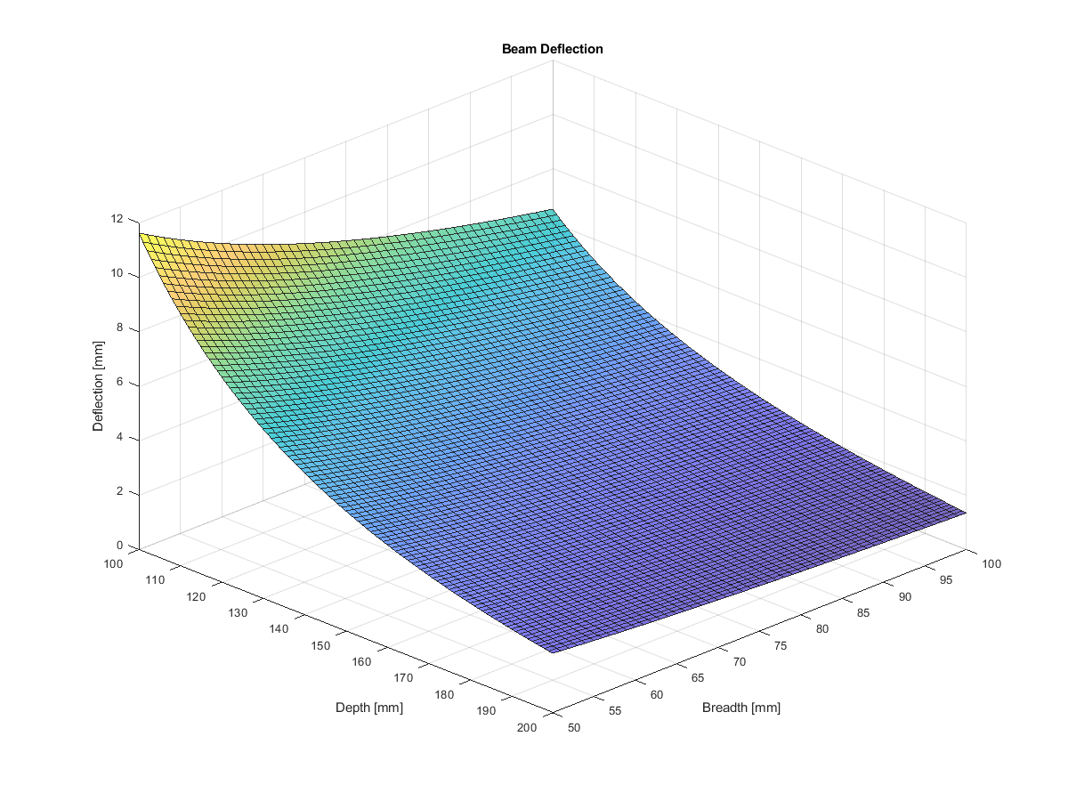
Unsurprisingly, that minimum occurs down on the bottom right hand corner as you look at the plot, where both depth and breadth are at their maximum.
We knew that going into this problem, but for more complex problems, we might not have such a clear idea of where the optimum solution lies before we start.
A better way
In a more realistic example, we might have a complex, multi-dimensional design space with an awkward shape, and we might not have any clear idea of where the best solution lies. Perhaps more importantly, real-world simulation cases can be incredibly complex,requiring vast HPC clusters and sometimes running for days. This is the scenario where we would definitely want to start using an optimisation routine to explore the design space for us, because anything even approaching an exhaustive search would be infeasible.
To bring this back to our beam example, instead of computing deflection at some quantised version of every possible $(b, d)$ pair, we would use an optimisation algorithm to explore the design space for us. We would start with an initial guess, compute the deflection at that point, then iteratively improve our guess until we arrive at the best solution.
Though we could use Nelder-Mead or similar methods mentioned above, this is where gradient-based optimisation like gradient descent come into play. We can use the gradient of our objective function with respect to our design variables to inform our next guess, and this can help us find the best solution more quickly.
Enter gradient descent
Ignoring the engineering scenarios for a moment, let’s consider a classic optimisation problem: Himmelblau’s function.
Himmelblau’s function exists entirely to test the performance of optimisation techniques. It’s a 2D function with four local minima and one local maximum, and it’s given by:
$$ f(x, y) = (x^2 + y - 11)^2 + (x + y^2 - 7)^2 $$
Over $x$ and $y$ ranges that span $[-4, 4]$, it looks like this:
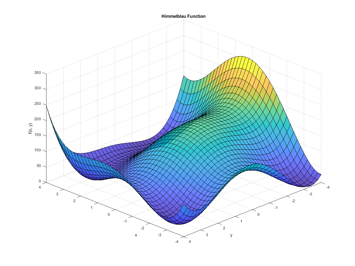
You can see the four minima and the maximum in the plot above, and you can see how the function’s surface is quite complex. Imagine something like this, but in ten or twenty dimensions, and you can see how it might rapidly become numerically impossible to sweep the entire range of possible solutions.
On gradient descent, the idea is to start at some initial position, then, over a series of iterations, move in the direction opposed to the direction of the objective function’s gradient vector. The gradient of your function at a given point is effectively pointing in the direction of steepest ascent, so it holds that the negative of the gradient points in the direction of steepest descent.
(For more information on why that’s actually the case, this, this, and this are all helpful.)
If we animate the path the algorithm takes as it moves towards a minimum, it looks like this:
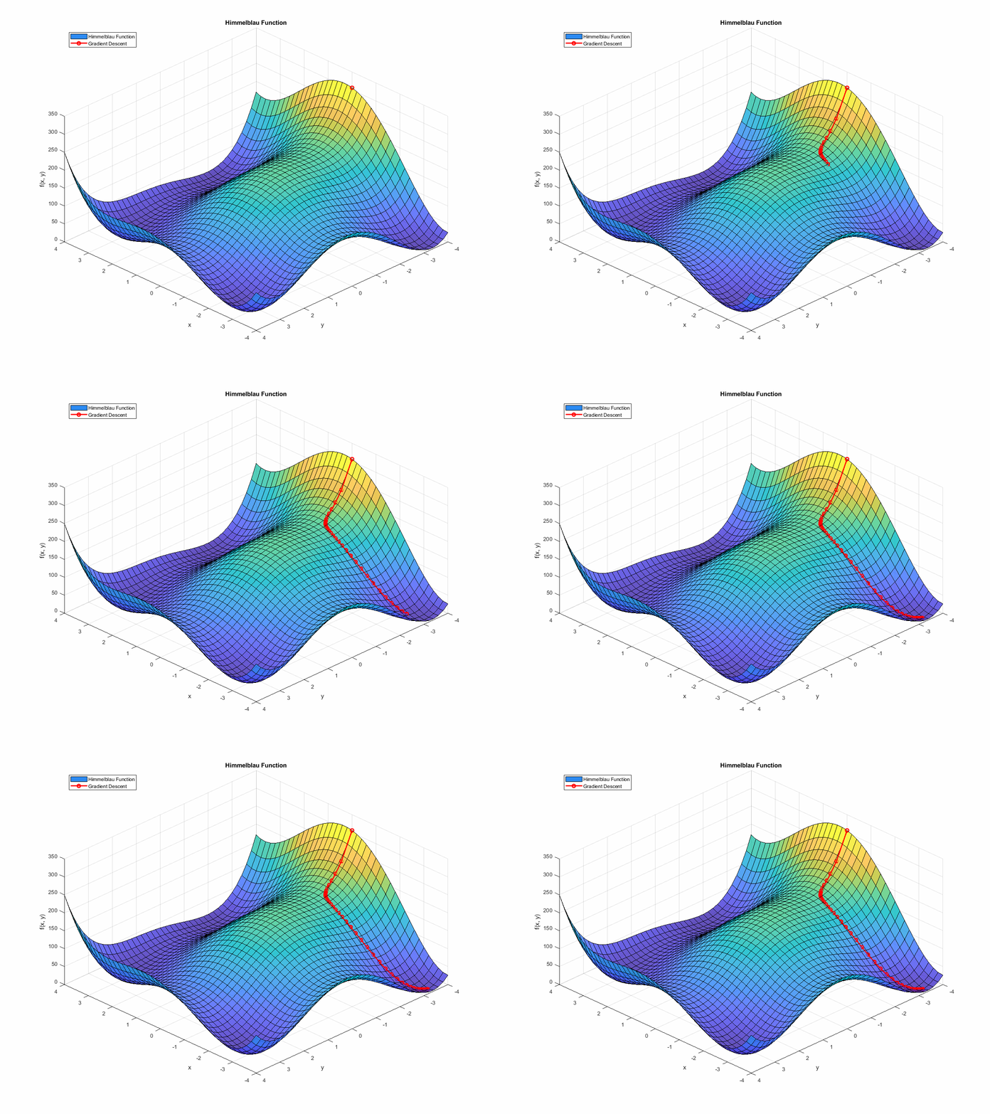
(If you’re interested in the code that generated this, it’s at the end of this post. You can find it here.)
Intro to gradient descent
This is likely familiar to many software and data people, so feel free to collapse this section and move on, but it may be interesting to any mechanical people reading...
The method is fairly straightforward:
- Pick a starting point.
- Select an initial position in the parameter space as the initial ‘guess’ for the location of the minimum.
- Note that the choice of the starting point can influence which minimum the algorithm converges to in functions with multiple minima.
- Compute the gradient of your function.
- Calculate the gradient of your objective function at the current point.
- This will be a vector that points in the direction of the steepest ascent of the function, and is given by the partial derivatives of the function with respect to each of its parameters.
- This partial derivative point is important, and something I’ll come back to later.
- Update the current point.
- Adjust current position, i.e. parameter values, by moving in the direction opposed to that of the gradient.
- This is achieved by first multiplying the gradient by a small scalar, called the learning rate, and then subtracting the result from the current point.
- In our example, we have two parameters, so we would expect to move both our $x$ and $y$ values—but in higher dimensions, we would be adjusting all of our parameters.
- Repeat until convergence.
- Repeat steps 2 and 3 until you reach some convergence criterion. This is typically when the norm of the gradient is less than some tolerance, indicating that you’re close to the minimum, when the change in the function value between iterations is less than some tolerance, or when you’ve reached some maximum number of iterations.
- In some cases, the evaluation of the function value at each point isn’t actually necessary for the algorithm to work. It can arrive at the optimum solution without it, but it is often useful to see how the function value changes as the algorithm progresses, and as above, some stopping criteria might be based on the function value.
The maths basically boils down to this:
$$x_{new} = x_{old} - \alpha \nabla f(x_{old})$$
Where:
- $x_{new}$ is the position vector at your next iteration.
- $x_{old}$ is the position vector at your current iteration.
- $\alpha$ is the learning rate.
- $\nabla f(x_{old})$ is the gradient of your function at your current position.
As stated above, the gradient will be a vector of partial derivatives. So if your vector $x = (x_1, x_2, x_3, … x_n)$, then your gradient will be a vector of partial derivatives, like this:
$$\nabla f(x) = \left[ \frac{\partial f}{\partial x_1}, \frac{\partial f}{\partial x_2}, \frac{\partial f}{\partial x_3}, … \frac{\partial f}{\partial x_n} \right]$$
Then, your stopping criteria is typically based on the norm of the gradient, like this:
$$ \lVert \nabla f(x) \rVert < \epsilon $$
Where:
- $\lVert \nabla f(x) \rVert$ is the norm or magnitude of the gradient vector.
- $\epsilon$ is your stopping tolerance.
If you’re like me and tend to find the Elvish symbols a bit less intuitive than code, I’d recommend checking the code given at the bottom of the post: here.
In search of partial derivatives
I mentioned above that the partial derivative point is important, and this is where the appeal of differentiable programming starts to raise its head. In order to make use of gradient-based optimisation, you need to compute the gradient of your objective function. To do that, you need to be able to compute the partial derivatives of your function with respect to each of its parameters.
Symbolic differentiation
In the case of the Himmelblau example above, we actually do this by hand—symbolically in the math-sy parlance. We have a simple expression, and we can compute its partial derivatives with respect to each of its parameters by hand, yielding two new expressions:
$$f(x, y) = (x^2 + y - 11)^2 + (x + y^2 - 7)^2$$ $$\frac{\partial f}{\partial x} = 2(2x(x^2 + y - 11) + x + y^2 - 7)$$ $$\frac{\partial f}{\partial y} = 2(2y(y^2 + x - 7) + y + x^2 - 11)$$
Then we can just drop this into our code and make a call to each of these functions to get the partial derivatives at each point:
% Define the Himmelblau function.
fHimmelblau = @(x, y) (x.^2 + y - 11).^2 + (x + y.^2 - 7).^2;
...
% Gradient of the function will be a vector of partial derivatives, but we
% can leave these as separate variables.
grad_fHimmelblau_x = @(x, y) 2*(2*x.*(x.^2 + y - 11) + x + y.^2 - 7); % df/dx
grad_fHimmelblau_y = @(x, y) 2*(x.^2 + 2*y.*(y.^2 + x - 7) - 11); % df/dy
This is straightforward for a function like Himmelblau’s, but this is not going to be replicated across many real engineering problems.
Numerical differentiation
As an alternative to testing your high school mathematics abilities, these terms can also be computed numerically. That means evaluating your function at some positions around your current point, and then using the results to estimate the partial derivatives—effectively by doing some variant of rise over run along each axis. This approach is particularly useful when the symbolic form of the derivative is difficult to work out, or when dealing with functions where only numerical evaluations are possible.
There are really three main methods for doing this:
- Forward difference.
- Backward difference.
- Central difference.
Forward difference
For a function $f(x,y)$, the partial derivatives can be approximated as follows: $$\frac{\partial f}{\partial x} \approx \frac{f(x + h, y) - f(x, y)}{h}$$ $$\frac{\partial f}{\partial y} \approx \frac{f(x, y + h) - f(x, y)}{h}$$
Where $h$ is some small step size. Effectively, you just step ‘forwards’ in both $x$ and $y$, work out the change in function value, and then divide by the step size to get an estimate of the gradient.
Backward difference
This is really the same as the forward difference, but you step ‘backwards’ in both $x$ and $y$: $$\frac{\partial f}{\partial x} \approx \frac{f(x, y) - f(x - h, y)}{h}$$ $$\frac{\partial f}{\partial y} \approx \frac{f(x, y) - f(x, y - h)}{h}$$
Central difference
Effectively a combination of the two above, the central difference method is given by stepping both forwards and backwards, and then taking the average of the two results. This is generally more accurate than the forward or backward difference methods, and is given by the following equations: $$\frac{\partial f}{\partial x} \approx \frac{f(x + h, y) - f(x - h, y)}{2h}$$ $$\frac{\partial f}{\partial y} \approx \frac{f(x, y + h) - f(x, y - h)}{2h}$$
Considerations
Numerical differentiation provides an ability to compute the gradient of basically any function. This is quite attractive, and it means you can use gradient-based optimisation on any function you like. However, if you have to make four calls to your function to compute the gradient at each point, and you’re doing this over a large number of points, and your function is computationally expensive, then this can become a significant bottleneck.
You can also find funny edge cases where the step size is too large or too small, with numerical precision, near boundaries, and with functions that are not smooth. This can lead to inaccurate estimates of the gradient, and can lead to the optimisation algorithm failing to converge.
Automatic differentiation
Automatic differentiation is a technique that allows you to compute the partial derivatives of any function with respect to any of its parameters. To borrow from Wikipedia:
Automatic differentiation exploits the fact that every computer calculation, no matter how complicated, executes a sequence of elementary arithmetic operations (addition, subtraction, multiplication, division, etc.) and elementary functions (exp, log, sin, cos, etc.). By applying the chain rule repeatedly to these operations, partial derivatives of arbitrary order can be computed automatically, accurately to working precision, and using at most a small constant factor of more arithmetic operations than the original program.
This sounds incredible. For a constant factor more operations, you can get the gradients of anything you like without having to manually differentiate your function, and without having to worry about the computational or edge case issues that come with numerical differentiation. It’s a technique that can effectively expose an analytically correct derivative (to numerical precision) for any function you like. No sums; free gradients.
There are a whole series of libraries that can do this for you, and they’re often used in machine learning and optimisation contexts. These include autodiff, autograd, jax, PyTorch, and auto-diff.
The technique also gets used in some engineering contexts already, including some motorsport applications. This PhD thesis, Optimal Control and Reinforcement Learning for Formula One Lap Simulation, makes use of PyTorch’s automatic differentiation capabilities to accelerate a collocation solve.
Forward and reverse mode
It’s worth touching on this as it becomes relevant later, but there are two main modes of automatic differentiation: forward mode and reverse mode. The best explanation of the difference between these two I’ve seen is this Stack Exchange post, but the short version is that they effectively just work through the chain rule in different orders,and this can result in different numbers of operations required to arrive at the result.
Forward mode:
In forward mode, differentiation progresses from the independent (input) variables towards the dependent (output) variables. It computes the derivative of each intermediate operation with respect to the input variables as it goes, effectively applying the chain rule from the inputs to the outputs.
This mode is more efficient when the number of inputs is small compared to the number of outputs. This is because it calculates derivatives in a single pass, one per input variable.
Reverse mode:
In reverse mode, the calc works backward from the output to the inputs. It first computes the value of the function with a forward pass, then tracks back through a reverse pass, applying the chain rule in reverse to compute the derivatives of the output with respect to each input variable.
This mode is more efficient dealing with functions that have a small number of outputs, like a scalar objective function, and a large number of inputs, like a big set of parameters. This is because it computes all partial derivatives with respect to the inputs in a single backward pass.
Trade-offs and terminology
The choice between these two depends on the size of your input and output. Reverse mode is generally more efficient for functions with many inputs but few outputs… think neural networks with a scalar loss function. Forward mode is generally preferred when you have more outputs than inputs, as it avoids the computational overhead associated with the reverse pass that could be computationally intensive.
It’s also worth noting that these things both go by other names in different domains and contexts. These include:
- Forward mode:
- Forward accumulation.
- Tangent mode.
- Bottom-up†.
- Reverse mode:
- Reverse accumulation.
- Adjoint mode.
- Top-down†.
- Backpropagation‡.
† According to Wikipedia, but I don’t think I’ve seen this written anywhere else.
‡ Common in the ML/AI space.
Back to our I-beam
In the section above, I outlined a simple example of a design optimisation problem, where we wanted to minimise peak deflection in a simply supported, centrally loaded I-beam. I then went on to outline how you might use gradient descent to find the best solution to a problem of similar nature.
That latter section ultimately led up to this declaration of a requirement for partial derivatives, with these enabling us to use gradient-based optimisation to find the best solution to our problem.
To GitHub
To provide something like a vaguely realistic example of how this might work, I’ve put together an incredibly simple
example repo. It makes use of auto-diff, wrapping a simple second
moment of area calc in a function that yields, with every call, the beam’s second moment of area and that second moment
of area’s gradient with respect to the beam’s geometrical parameters.
The relevant code we can actually work through here.
This function returns the area moment of inertia of the specified section, $I_{xx}$:
def compute_area_moment_of_inertia(
    depth: float,
    width: float,
    t_web: float,
    t_flange: float,
) -> float:
    """
    Compute the area moment of inertia of an I-beam cross-section.

    Ref: https://www.engineeringtoolbox.com/area-moment-inertia-d_1328.html

    Args:
        depth (float): The depth of the section.
        width (float): The width of the section.
        t_web (float): The thickness of the section's web.
        t_flange (float): The thickness of the section's flange.

    Returns:
        float: The area moment of inertia of the beam cross-section.
    """
    depth_web = depth - 2 * t_flange
    moi_x = (t_web * depth_web**3 / 12) + (width / 12) * (depth**3 - depth_web**3)

    return moi_x
This simple function unwraps an array and passes it into the compute_area_moment_of_inertia function:
def compute_area_moment_of_inertia_ad(x: np.ndarray) -> np.ndarray:
    """
    Wraps the compute_area_moment_of_inertia function to accept an array of inputs.

    Args:
        x (np.ndarray): An array of inputs containing the dimensions of the object.

    Returns:
        np.ndarray: The computed area moment of inertia.
    """
    return compute_area_moment_of_inertia(x[0], x[1], x[2], x[3])
While this function actually handles the automatic differentiation:
def compute_area_moment_of_inertia_sensitivities(
    depth: float,
    width: float,
    t_web: float,
    t_flange: float,
):
    """
    Compute the area moment of inertia and sensitivities for a given set of parameters.

    Args:
        depth (float): The depth of the section.
        width (float): The width of the section.
        t_web (float): The thickness of the section's web.
        t_flange (float): The thickness of the section's flange.

    Returns:
        tuple: A tuple containing the area moment of inertia and sensitivities.
               The area moment of inertia is a scalar value.
               The sensitivities are a list of derivatives with respect to the input parameters.
    """
    x = np.array([[depth], [width], [t_web], [t_flange]])

    with auto_diff.AutoDiff(x) as x:
        moi_x = compute_area_moment_of_inertia_ad(x)

    moi = moi_x.val[0]

    # We only have one output, so the list of lists of lists can be flattened to a simple list.
    sensitivities_raw = moi_x.der.tolist()
    sensitivities = [x[0] for x in sensitivities_raw[0]]

    return (moi, sensitivities)
This final one is the interesting one. We can make a very simple call to this function and get some interesting outputs.
Say we called compute_area_moment_of_inertia_sensitivities(100, 40, 5, 5), that would give us not just the area moment
of inertia of the section, but also the sensitivities of that area moment of inertia with respect to each of the values
we’ve passed in.
If I place a breakpoint in the right spot, we can take a look at what we get here:
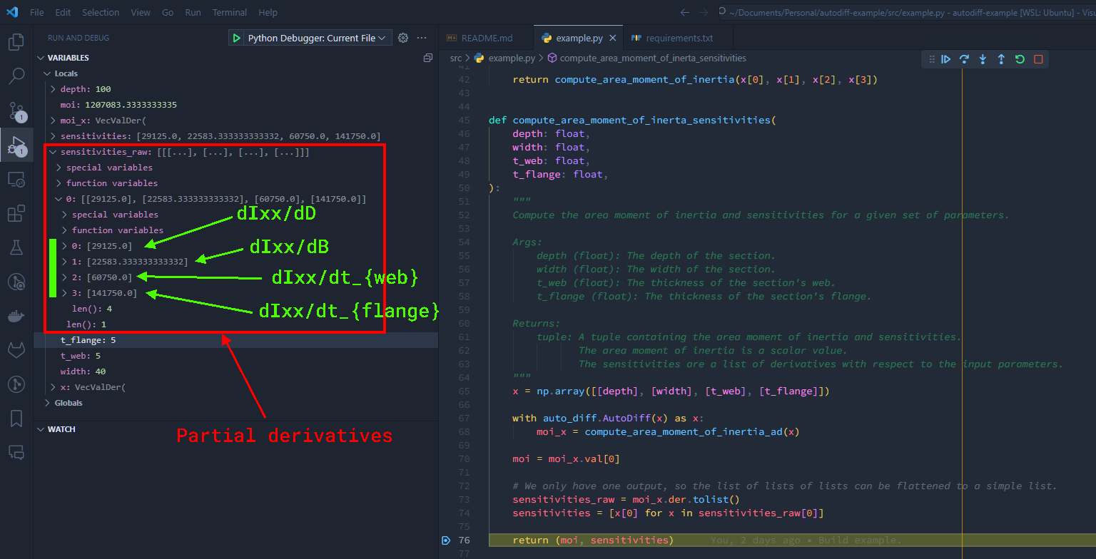
Already, I’m seeing things I didn’t expect. Even though it’s an I-beam and not a solid square section, I think of the second moment of area of something like this being basically $bd^3/12$, so I would expect the second moment of area to be most sensitive to changes in depth. However, looking at the values we get out here, it’s actually most sensitive to changes in flange thickness.
This is an interesting way to force yourself to think, as after ruminating on this for a minute or two, it makes perfect sense. Each of the flanges is as far from the centroid of the section as you can get, so changes in flange thickness will have a greater effect on the second moment of area—plus there’s one at the top and one at the bottom, so a 1mm adjustment in our flange thickness value will result in two flanges each getting 1mm thicker.
However, that’s sort of beside the point. Here, what you can see is that I have a function that can compute the second moment of area of an I-beam section, and that will also give the partial derivatives of that value with respect to each of the section’s parameters that we pass in. This is exactly what we were after to enable gradient-based optimisation.
Look at it go
In this case, we can’t directly use simple gradient descent to find the best I-beam section, because we have a set of constraints that we need to satisfy.
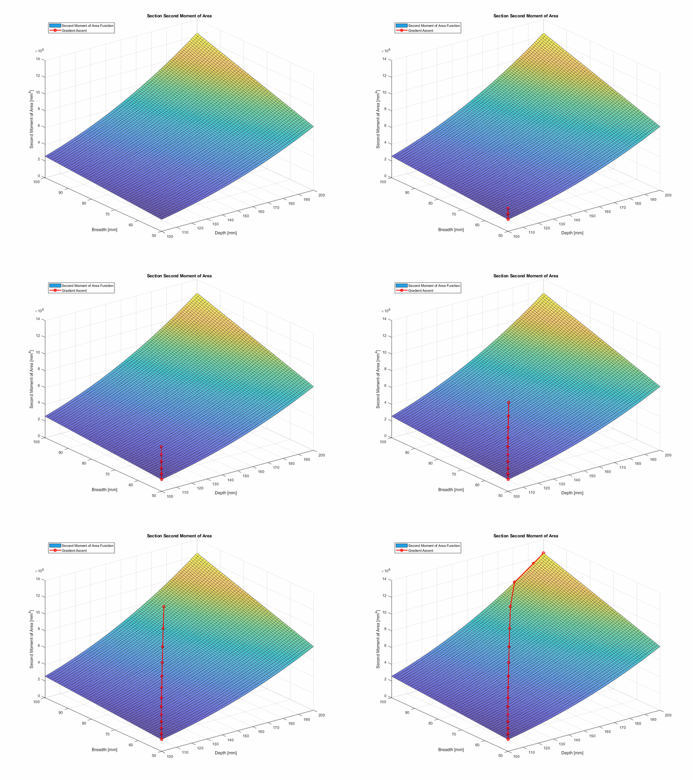
However, we can build on the technique, using something known as projected gradient descent (which is really gradient ascent in this case). With projected gradient descent, we can use the gradients to inform our next guess, and then project that guess back into the feasible space,allowing us to avoid the solution space that would violate our constraints.
In the interest of simplicity, I’ve chopped out the deflection component. So, instead of minimising deflection, we’re maximising second moment of area—which will achieve the same thing.
This method actually works very nicely. You can find the code for this in the run_gradient_ascent function
in the repo, and you can see it in action
here… telling you what a first year engineering student could tell you without a moment’s hesitation, but with more
steps:
Summary
I hope that all makes sense. The provided example shows how automatic differentiation lets us get analytically correct partial derivatives of a function we might be interested in, without having to compute any derivatives by hand, then it shows how we might use those partial derivatives in combination with some optimisation method to arrive at a good solution to vaguely realistic engineering design optimisation problem.
Real design processes
I find this stuff incredibly interesting, but let’s work through some examples of how things might work for real.
Manual design optimisation
Unfortunately, the I-beam example above is not very representative of a real-world workflow. In a real engineering team, where you run a mix of tools from Dassault and Ansys and Siemens and whoever else, you don’t typically have hand-coded geometry creation functions, hand-coded moment of inertia and deflection equations, and a simple 2D design space. Instead, you have a complex mix of often siloed products, with friction-heavy interfaces, no ability to wrap things in automatic differentiation libraries, and no straightforward way of closing the loop between CAD and simulation.
As a result, your actual process will probably be more like this:
- Do some initial calcs or analytical simulation to set your initial parameters.
- Build a CAD model with those parameters.
- Load that geometry into the relevant tool, pre-process/build/tweak/refine a mesh to fit your needs, and set your simulation running.
- Once the simulation has finished, extract/post-process the relevant results and manually analyse them.
- This could involve manual interrogation of flow velocity or pressure plots, identification of stress concentrations in particular areas of the geometry, extraction of peak stresses or deflections etc.
- Using engineering judgement, tweak the CAD to address any of the more pressing issues you’ve identified, then go back
to step 3 and repeat the process.
- If you’re lucky, you might have some variety of simplified model from step 1 that you can adjust to correlate with your simulation results, and then use that to inform your next iteration of the CAD model.
- Simulation results are also largely best compared to other simulation results, so you might have to run a few iterations of this process to be happy with how your design is performing.
Parametric design optimisation
Taking the above manual process and applying some more structure to it leads you to what we might call ‘parametric design optimisation’. Here, as above, you start with some initial calcs or analytical simulation to set your initial parameters, and once again you build a parametric CAD model that can be adjusted.
However, instead of manually running and interrogating simulation results and using engineering judgement to inform your next iteration, you apply an optimisation tool and leverage that to home in on your optimum design. There are commercial tools out there for this already, like Ansys optiSLang.
Ignoring the option to integrate multiple simulation tools, the process here is effectively the same as above, but with the software handling steps 3 to 5:
- Do some initial calcs or analytical simulation to set your initial parameters.
- Build a CAD model with those parameters.
- Load that geometry into the relevant tool and pre-process/build/tweak/refine a mesh to fit your needs.
- Tell your optimisation tool what your objective is, how it can invoke your simulation, and what your constraints are.
- Let it run, building the simulations and running them, and interrogating the results—ultimately examining the design space and iterating on the best solution.
This approach can also be used to spit out some sensitivity analysis, letting you retain some understanding of how your system performance will respond to changes in its design.
Adjoint methods
As touched on above, ‘adjoint mode’ is another name for reverse mode automatic differentiation. This technique gives us inexpensive gradient calculation; inexpensive in that we don’t have to spend time manually deriving derivatives, and inexpensive in that we can extract analytically correct derivatives across a large number of input variables with a single simulation run.
In the context of simulation-driven design optimisation, this is an attractive proposition. Unlike with the parametric design optimisation approach, where you might have to run a large number of simulations to explore the design space, the adjoint method lets you run a significantly smaller number of simulations, but still extract partial derivatives for a large number of input variables.
Adjoint optimisation and sensitivity analysis
Taking a wing as an example again, let’s say we have an initial geometry defined, and we want to use simulation to help us steer some modification to the profile for increased lift. First, we’ll configure a domain for the simulation,configuring both a volume mesh and a surface mesh. If we’re interested in knowing how we should change the shape of the thing to increase our lift, we’re going to want some kind of sensitivity data to tell us where we should first look to make changes.
Helpfully, this is exactly what our adjoint method will provide us with: a CFD solution from the ‘primal’ simulation, and a set of partial derivatives that will tell us what the overall lift sensitivity is to a small positional change of every point on the surface mesh.
This exact process is described in the context of morphing aerostructures in the paper Fast Sensitivity Analysis for the Design of Morphing Airfoils at Different Frequency Regimes by Kramer, Fuchs, Knacke, et. al. For our argument here, we aren’t really interested in the frequency component of the problem, so I’ll butcher a single case and annotate it with some of the things we might be interested in:
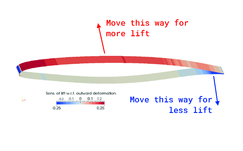
Adapted from Kramer, Fuchs, Knacke, et. al.
Basically, what this is showing us is that we have a set of partial derivatives that we can map onto our geometry that tell us how we need to change the the foil profile to increase lift. This is exactly the kind of data we would want to inform our next iteration of the design, given that our objective was to increase lift.
If we were to have attempted something like this with a parametric design optimisation tool, we would have had to run a number of simulations with modified geometries in order to explore the design space, and then we would have had to compute the differences in lift between each of those simulations to inform our next iteration of the design. Given that the computational cost of a single CFD simulation can be quite high, this could be a very expensive process, particularly when the adjoint method can give us that information with a single simulation run.
Shape modification
These sensitivities can also be used to inform and drive automated shape modification, effectively letting the solver drive the design process. Another mention for Ansys here, as they already offer adjoint shape optimisation tools for CFD, including ‘mesh morphing’ that can perform shape modification based on the sensitivities extracted from an adjoint solve.
Here’s a figure reproduced from an Ansys presentation by Franklyn Kelecy—note the ‘mesh morph’ step on the left hand side:
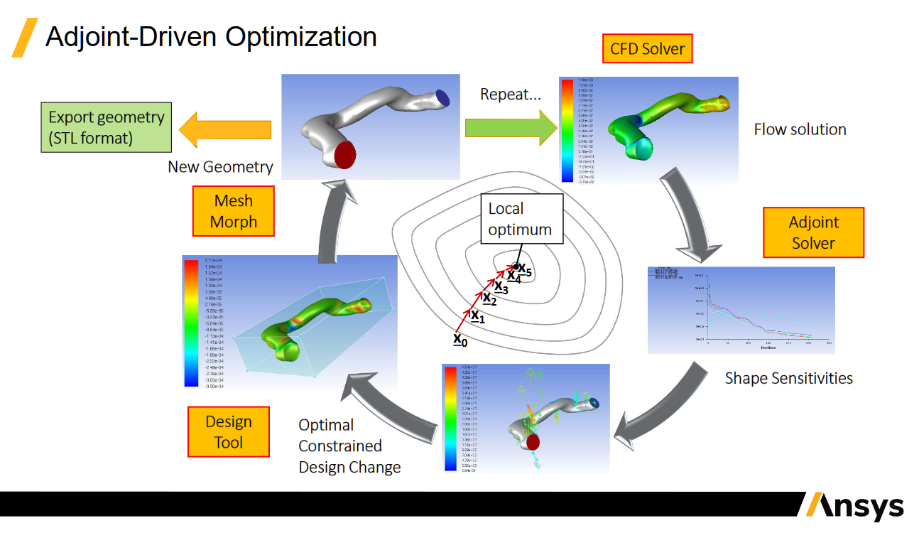
Credit: Adjoint Shape Optimization for Aerospace Applications
Practically, this allows for mesh deformation and exploration of alternate geometries without having to adjust a CAD model, and without having to regenerate a mesh that’s derived from that CAD model.
This is incredible. We already have commercially available tools out there that let component geometries be plugged into some sort of optimisation routine, and that iteratively improve upon a part’s design without significant human input… all making use of adjoint sensitivities to inform the next iteration of the design.
Wait, it’s all optimisation?

Given all of that, we’ve basically come full circle. The end goal of all the maths and the plots and the computational techniques discussed was really just to get some sensitivity values. These values are then used to help iteratively improve a design and improve the performance of some system, just like the teams of human engineers with some simplified mental models of these things have been doing all along.
So, it has always been optimisation, but computation lets us do it faster, and more robustly, and with more complex systems. It lets us do it with more parameters, and with more complex objectives, and with more complex constraints. It lets us do it with less human input, less human error, and less human bias… and in the case of differentiable programming, it lets us do all of that with less computational cost.
CAD and differentiable programming
I’ve been talking about this stuff in the context of simplified, hand-coded examples, and of CFD and FEA, but made next to no mention of CAD thus far. This has been intentional, as I think it would be incredibly confusing to just start talking about differentiable CAD and new CAD kernels without first working through what differentiable programming actually is, how engineering problems can be thought of as optimisation problems, and how simulation-heavy engineering processes typically work.
In general, I think differentiable programming is an incredibly interesting area, and it’s already being used all over the place, including in engineering tools that are already on the market. In the CFD and FEA cases, it’s pretty incredible to be able to extract such granular sensitivity data from a single simulation run, and to be able to use that data to steer the design process.
How this might be applied to CAD is a bit less clear to me, but I think I can see the grander vision where the appeal truly lies.
In isolation
In isolation, I don’t think I see much value in building a differentiable CAD system. If our goals relate to optimisation and iterative design improvement and closed-loop, simulation-driven design processes, then I struggle to see which parameters that the CAD system ‘owns’ are really of interest. CAD packages are specialised tools for geometry creation, and as a result, the parameters that they own are effectively all geometrical properties, though perhaps with a density value thrown in. Your CAD system can tell you things like lengths, areas, volumes, masses, moments of inertia, and so on, so with automatic differentiation thrown in, it could tell you how these things relate to driving parameters. However, it can’t tell you things like lift, drag, stress, deflection, pressure drop, natural frequency… or any of the other performance-oriented metrics that you might actually be interested in minimising or maximising.
Of course, there are some relatively direct relationships between these things and the quantities we would actually want to solve for, but often these relationships are complex and non-linear, and your CAD system really knows nothing about them at all.
Perhaps the selling point here would be more closely related to the geometrical considerations that relate to manufacturing and packaging than to performance, but that sits well outside anything I’ve ever worked on.
In an end-to-end differentiable ecosystem
I think this is the grand vision. If, as they can already, your simulation tools can run both primal and adjoint solves, giving you sensitivities to the millions of input parameters that you might have in a complex mesh, then you can relate those sensitivities back to the input parameters that drive your CAD model.
With end-to-end support for differentiable everything, instead of asking “How would lift respond to some infinitesimally small change in the $(x,y,z)$ coordinate of some node on the surface of my wing?”, as existing adjoint methods allow, you can ask how lift would respond to a change in camber, or chord length, or twist, or thickness, or any of the other parameters that you might have that actually drive your CAD model’s geometry.
Practically, I don’t know how the hand-off of these derivatives would work. I imagine there would need to be a derivative interface between the CAD and the meshing and the simulation tools, and that you would need to be able to relate CAD parameters to the mesh, and then the mesh to the simulation results, and then the simulation results back to the CAD parameters—but I think this should be soluble.
If that were achievable, it would allow not just for free-form mesh morphing that is unlikely to be directly applicable to critical features like those of bearings and shafts, but for computationally efficient, structured design optimisation. It would allow for the closed-loop, simulation-driven design process to adjust diameters and eccentricities and chord lengths and so on, all while homing in on the best possible solution to the problem at hand in as few simulation runs as possible.
Alternatives
Interestingly, there is a paper from my old department at QUB, Linking Parametric CAD with Adjoint Surface Sensitivities, that presents a method of combining adjoint methods with contemporary, non-differentiable parametric CAD.
This approach does require perturbation of the CAD model, but they still report a computationally efficient mechanism for arriving at parametric sensitivities.
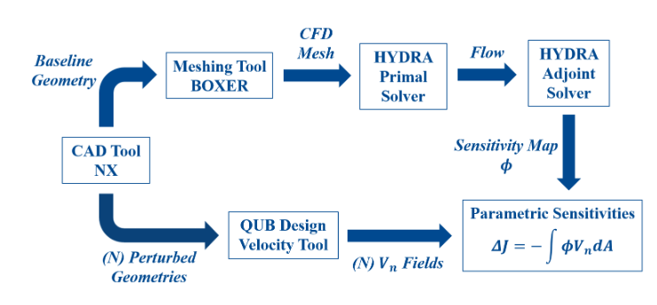
Credit: Vasilopoulos, Agarwal, Meyer et. al.
Conclusion
My broad view is that differentiable programming offers some exciting use cases in engineering, but I don’t think we would see the full benefit of this until we arrive at some sort of end-to-end (eco)system that accommodates the paradigm.
I’m a big fan of open and interoperable tools, so I hope this goes the way of some sort of standard that allows for straightforward integration of different systems,wholly unlike the history of commercial CAD systems to date.
Limitations
The biggest limitation I see is probably just the frequently non-linear nature of the relationships between the parameters that the CAD system owns and the quantities that we actually care about. I imagine you get around this with appropriate configuration of any optimisation technique, but I think it’s worth noting that your objective function could be highly non-linear, and that this could cause issues with gradient-based optimisation failing to converge, getting trapped in local minima, and so on.
It could also be challenging to employ adjoint methods with a large number of output parameters, as the reverse mode automatic differentiation technique is generally more efficient when the number of inputs is small
Disclaimer
I should probably say that I’m not really an expert on any of this stuff, so it is entirely possible that there are inaccurate comments and misunderstandings here.
However, I do straddle the worlds of both mechanical engineering and software development. I’ve battled with ancient versions of CATIA, designed bits of engines, developed new suspension systems, and built a lot of scientific/mathematical software, so I have quite a lot of exposure to the tools and techniques that are discussed here.
I hope that any overly shallow knowledge hasn’t detracted from the overall message, but if you spot any egregious errors, please just get in touch and let me know.
Appendix
Papers, reports, presentations etc.
Some of these provide some interesting background, alternative techniques etc.
- Linking Parametric CAD with Adjoint Surface Sensitivities
- Differentiable 3D CAD Programs for Bidirectional Editing
- Design Sensitivity Calculations Directly on CAD-based Geometry
- Adjoint Shape Optimization for Aerospace Applications
- Optimal Control and Reinforcement Learning for Formula One Lap Simulation
- Using Automatic Differentation for Adjoint CFD Code Developent
- Fast Sensitivity Analysis for the Design of Morphing Airfoils at Different Frequency Regimes
Videos
This video, You Should Be Using Automatic Differentiation, is probably worth watching:
Coincidentally, Ryan was also an advisor to Quant Insight while I was there, and the website would suggest he’s still active in that position.
These are good examples of adjoint methods in action:
Code
MATLAB Himmelblau function and gradient descent
This will generate the Himmelblau function and animate the path of a gradient descent algorithm as it moves towards a local minimum.
This is in MATLAB because the Windows/WSL2 combo I’m currently running doesn’t play well with matplotlib.
%% Initial setup.
OUTPUT_FILENAME = 'HimmelblauGradientDescentAnimation.gif';

% Define the Himmelblau function.
fHimmelblau = @(x, y) (x.^2 + y - 11).^2 + (x + y.^2 - 7).^2;

% Build the surface we'll plot gradient descent across.
xRange = -4:0.2:4;
yRange = -4:0.2:4;
[xGrid, yGrid] = meshgrid(xRange, yRange);
zValues = arrayfun(fHimmelblau, xGrid, yGrid);

% Plot.
hFigure = figure("Position", [500, 200, 1200, 900], 'Color', 'w');
hAx = axes(hFigure);
hSurf = surf(hAx, xGrid, yGrid, zValues, 'FaceAlpha', 0.8);
xlabel('x');
ylabel('y');
zlabel('f(x, y)');
hold on;
title('Himmelblau Function');
set(hAx, 'View', [-135, 45]);

%% Gradient descent.

% Gradient of the function will be a vector of partial derivatives, but we
% can leave these as separate variables.
grad_fHimmelblau_x = @(x, y) 2*(2*x.*(x.^2 + y - 11) + x + y.^2 - 7); % df/dx
grad_fHimmelblau_y = @(x, y) 2*(x.^2 + 2*y.*(y.^2 + x - 7) - 11); % df/dy

% Set gradient descent parameters.
ALPHA = 0.003; % Learning rate.
MAX_ITER = 200; % Maximum number of iterations.
SOLVE_TOLERANCE = 1e-3; % Tolerance for stopping criterion.

% Preallocate gradient descent path vectors.
pathX = NaN(MAX_ITER, 1);
pathY = NaN(MAX_ITER, 1);
pathZ = NaN(MAX_ITER, 1);

% Initial 'guess'.
x = 0; % Initial x value.
y = -4; % Initial y value.
z = fHimmelblau(x, y); % Initial z value.

pathX(1) = x;
pathY(1) = y;
pathZ(1) = z;

% Add to plot.
DELAY_TIME = 0.05; % Animation frame hold time.
hGradientDescent = plot3(hAx, pathX, pathY, pathZ, 'r-', 'LineWidth', 2, 'Marker', 'o');
hLegend = legend([hSurf, hGradientDescent], 'Himmelblau Function', 'Gradient Descent', 'location', 'NorthWest');

% Write initial frame.
frame = getframe(gcf);
im = frame2im(frame);
[imind, cm] = rgb2ind(im, 256);
imwrite(imind, cm, OUTPUT_FILENAME, 'gif', 'Loopcount', inf, 'DelayTime', DELAY_TIME);

% Solve.
for iter = 1:MAX_ITER
    % Compute gradient.
    gradX = grad_fHimmelblau_x(x, y);
    gradY = grad_fHimmelblau_y(x, y);

    % Update x and y by moving in the direction opposite to the gradient.
    x = x - ALPHA * gradX;
    y = y - ALPHA * gradY;
    z = fHimmelblau(x, y);

    % Store the path.
    pathX(iter + 1) = x;
    pathY(iter + 1) = y;
    pathZ(iter + 1) = z;

    % Update plot.
    set(hGradientDescent, 'xdata', pathX, 'ydata', pathY, 'zdata', pathZ);

    % Capture the frame
    drawnow;
    frame = getframe(gcf);
    im = frame2im(frame);
    [imind, cm] = rgb2ind(im, 256);

    % Write out.
    imwrite(imind, cm, OUTPUT_FILENAME, 'gif', 'WriteMode', 'append', 'DelayTime', DELAY_TIME);

    % Check for convergence.
    if norm([gradX, gradY]) < SOLVE_TOLERANCE
        break;
    end
end